кё°ліём ҒмңјлЎң м•„лһҳмІҳлҹј н•ңлӢӨ.
cname <- c("x1", "x2", "x3","x4", "x5", "x6", "y")
german = read.table("c:\\data\\german1.txt", col.names = cname)
options(contrasts = c("contr.treatment", "contr.poly"))
german.object <- glm(y~.,family=binomial, data=german)
summary(german.object)
p <- predict(german.object, german, type="response")
german <- cbind(german, p)
head(german)
pлҠ” y=1мқј нҷ•лҘ мқҙлӢӨ. көҗм ңм—җм„ңлҠ” y=1мқҙ л¶Ҳлҹүкі к°қмқҙлӢӨ.
> head(german)
   x1 x2  x3 x4 x5 x6 y          p
1 A11  6 A34  4 67  1 0 0.18170622
2 A12 48 A32  2 22  1 1 0.63312134
3 A14 12 A34  3 49  2 0 0.04812842
4 A11 42 A32  4 45  2 0 0.64393801
5 A11 24 A33  4 53  2 1 0.47102819
6 A14 36 A32  4 35  2 0 0.20127115
4 ліҖмҲҳм„ нғқлІ• #
м „м§„м„ нғқ, ліҖмҲҳмҶҢкұ°, л‘ҳлӢӨ
cname <- c("x1", "x2", "x3","x4", "x5", "x6", "y")
german = read.table("c:\\data\\german1.txt", col.names = cname)
#мғҒмҲҳн•ӯл§Ң нҸ¬н•Ён•ң мҙҲкё°лӘЁнҳ•
g.object <- glm(y~1, family=binomial, data=german)
#м „м§„м„ нғқлІ•
s.list <- list(upper = update(g.object, ~. +x1+x2+x3+x4+x5+x6))
step(g.object, scope=s.list, direction="forward")
#ліҖмҲҳмҶҢкұ°лІ•
#s.list <- list(lower = update(g.object, ~. -x1-x2-x3-x4-x5-x6))
#step(g.object, scope=s.list, direction="backward")
#л‘ҳлӢӨ
#s.list <- list(upper = update(g.object, ~. +x1+x2+x3+x4+x5+x6), lower = update(g.object, ~. -x1-x2-x3-x4-x5-x6))
#step(g.object, scope=s.list, direction="both")
кІ°кіј
> step(g.object, scope=s.list, direction="forward")
Start:  AIC=1223.73
y ~ 1

       Df Deviance    AIC
+ x1    3   1090.4 1098.4
+ x3    4   1161.3 1171.3
+ x2    1   1177.1 1181.1
+ x5    1   1213.1 1217.1
<none>      1221.7 1223.7
+ x6    1   1221.7 1225.7
+ x4    1   1221.7 1225.7

Step:  AIC=1098.39
y ~ x1

       Df Deviance    AIC
+ x2    1   1051.9 1061.9
+ x3    4   1053.2 1069.2
+ x5    1   1085.0 1095.0
<none>      1090.4 1098.4
+ x4    1   1090.2 1100.2
+ x6    1   1090.3 1100.3

Step:  AIC=1061.9
y ~ x1 + x2

       Df Deviance    AIC
+ x3    4   1022.6 1040.6
+ x5    1   1046.7 1058.7
<none>      1051.9 1061.9
+ x4    1   1051.5 1063.5
+ x6    1   1051.9 1063.9

Step:  AIC=1040.58
y ~ x1 + x2 + x3

       Df Deviance    AIC
+ x5    1   1019.3 1039.3
<none>      1022.6 1040.6
+ x6    1   1022.5 1042.5
+ x4    1   1022.5 1042.5

Step:  AIC=1039.27
y ~ x1 + x2 + x3 + x5

       Df Deviance    AIC
<none>      1019.3 1039.3
+ x4    1   1019.2 1041.2
+ x6    1   1019.3 1041.3

Call:  glm(formula = y ~ x1 + x2 + x3 + x5, family = binomial, data = german)

Coefficients:
(Intercept)        x1A12        x1A13        x1A14           x2
    0.66510     -0.53186     -1.07608     -1.89880      0.03434
      x3A31        x3A32        x3A33        x3A34           x5
   -0.09915     -0.94696     -0.93433     -1.52607     -0.01277

Degrees of Freedom: 999 Total (i.e. Null);  990 Residual
Null Deviance:	    1222
Residual Deviance: 1019 	AIC: 1039
>
мөңмў…м ҒмңјлЎң glm(formula = y ~ x1 + x2 + x3 + x5, family = binomial, data = german) к°Җ м„ нғқлҗҳм—ҲлӢӨ. AICк°Җ к°ҖмһҘ м ҒмқҖ лӘЁлҚёмқҙ м„ нғқлҗңлӢӨ.
м°ёкі : AIC (
![[http]](/moniwiki/imgs/http.png) м¶ңмІҳ(http://blog.naver.com/pinokio129?Redirect=Log&logNo=80018702687)
м¶ңмІҳ(http://blog.naver.com/pinokio129?Redirect=Log&logNo=80018702687))
AIC нҶөкі„лҹү
мөңм Ғ лӘЁнҳ•мқ„ кІ°м •н•ҳлҠ” кІҪмҡ° лӘЁнҳ•мқҳ м„ӨлӘ…лҠҘл Ҙкіј лӘЁнҳ•мқҳ м Ҳм•Ҫм„ұмқ„ кі л Өн•ҙм•ј н•Ё.
лӘЁнҳ•мқҳ м„ӨлӘ…лҠҘл ҘмқҖ мҡ°лҸ„(likelihood)лЎңм„ң мёЎм •лҗ мҲҳ мһҲмңјл©°,
лӘЁнҳ•мқҳ м Ҳм•Ҫм„ұмқҖ ліөмһЎн•ң лӘЁнҳ• ліҙлӢӨлҠ” к°„кІ°н•ң лӘЁнҳ•мқҙ м„ нҳёлҗҳм–ҙм•ј н•ңлӢӨлҠ” кІғмңјлЎң
м¶”м • кі„мҲҳмқҳ ж•ёк°Җ л§ҺмқҖ кІғм—җ лҢҖн•ҙ лІҢм№ҷмқ„ к°Җн•ЁмңјлЎңмҚЁ кі л Өлҗ мҲҳ мһҲлӢӨ.
к·ёлҹ¬лӮҳ лӘЁнҳ•мқҳ м„ӨлӘ…л Ҙкіј м Ҳм•Ҫм„ұмқҖ мғҒ충лҗҳлҠ”(trade-off)кё°мӨҖмңјлЎңм„ң,
мҷ•мҷ• ліөмһЎн•ң лӘЁнҳ•мқҙ м„ӨлӘ…л Ҙмқҙ нҒ°кІғмқ„ л°ңкІ¬ н• мҲҳ мһҲлӢӨ.
л”°лқјм„ң л‘җ нҢҗлӢЁкё°мӨҖмқ„ н•Ёк»ҳ кі л Өн•ң м„ нғқк·ңмӨҖмқҙ н•„мҡ”н•ҳкІҢ лҗңлӢӨ.
к·ёкІғмқҙ л°”лЎң м •ліҙкё°мӨҖ м ‘к·јлІ•мңјлЎң Akailkeм—җ мқҳн•ҳм—¬ к°ңл°ңлҗң
Akaike Information Criterion(AIC)мқҙлӢӨ.
AIC = -2 log L +2n
м—¬кё°м„ң 'n': нҢҢлқјлҜён„° мҲҳлҘј лӮҳнғҖлӮҙл©°, 'log L'мқҖ лҢҖмҲҳмҡ°лҸ„(log-likelihood).
вҖ» Akailkeм—җ мқҳн•ҳл©ҙ AICнҶөкі„лҹүмқҳ к°’мқҙ мөңмҶҢк°Җ лҗҳлҠ” лӘЁнҳ•мқ„ мұ„нғқн•ҳм—¬м•ј лҗңлӢӨ
D(Deviance)лҠ” мқјл°ҳнҷ”лҗң м„ нҳ• лӘЁнҳ•м—җм„ң лӘЁнҳ•мқҳ м Ғн•©лҸ„ кІҖмҰқ нҶөлҹүмқҙлӢӨ.
cname <- c("x1", "x2", "x3","x4", "x5", "x6", "y")
german = read.table("c:\\data\\german1.txt", col.names = cname)
options(contrasts = c("contr.treatment", "contr.poly"))
german.object <- glm(formula = y ~ x1 + x2 + x3 + x5, family = binomial, data = german)
summary(german.object)
кІ°кіј
Call:
glm(formula = y ~ x1 + x2 + x3 + x5, family = binomial, data = german)
Deviance Residuals:
Min 1Q Median 3Q Max
-1.7997 -0.8007 -0.4747 0.9283 2.4241
Coefficients:
Estimate Std. Error z value Pr(>|z|)
(Intercept) 0.665099 0.476311 1.396 0.162607
x1A12 -0.531864 0.185402 -2.869 0.004121 **
x1A13 -1.076082 0.336956 -3.194 0.001405 **
x1A14 -1.898800 0.206314 -9.203 < 2e-16 ***
x2 0.034342 0.006329 5.426 5.76e-08 ***
x3A31 -0.099153 0.474942 -0.209 0.834629
x3A32 -0.946961 0.370644 -2.555 0.010622 *
x3A33 -0.934327 0.433303 -2.156 0.031061 *
x3A34 -1.526069 0.393754 -3.876 0.000106 ***
x5 -0.012765 0.007091 -1.800 0.071821 .
---
Signif. codes: 0 вҖҳ***вҖҷ 0.001 вҖҳ**вҖҷ 0.01 вҖҳ*вҖҷ 0.05 вҖҳ.вҖҷ 0.1 вҖҳ вҖҷ 1
(Dispersion parameter for binomial family taken to be 1)
Null deviance: 1221.7 on 999 degrees of freedom
Residual deviance: 1019.3 on 990 degrees of freedom
AIC: 1039.3
Number of Fisher Scoring iterations: 4
мҲ«мһҗнҳ• ліҖмҲҳмқё кІҪмҡ° 분нҸ¬лҘј ліҙкі нӣ„ліҙлҘј м„ нғқн• мҲҳ мһҲлӢӨ. (YлӢҳмқҙ м•Ңл ӨмӨҖкұ°лӢӨ)
# r: кІ°кіјset
# rм—җм„ң мҲ«мһҗнҳ• мһҗлЈҢл§Ң м„ лі„н•ҙм„ң plotting
# columnмқҙ мҲ«мһҗнҳ•мқём§Җ T/F м ҖмһҘ
training <- sqlQuery(conn, "select
cnt x1
, logkind x4
, genre x5
, diff_cnt x6
, diff_time x8
, gamecd x9
, reg_hh x10
, case when t <= 2 then 1 else 0 end y
from temp.dbo.out_data01
")
#install.packages("reshape")
#install.packages("ggplot2")
library("reshape")
library("ggplot2")
number_cols <- sapply(training, is.numeric)
r.lng <- melt(training[,number_cols], id="y") # id: мў…мҶҚліҖмҲҳлӘ….
p <- ggplot(aes(x=value, group=y, colour=factor(y)), data=r.lng)
p + geom_density() + facet_wrap(~variable,scale="free")
кІ°кіјлҠ” лӢӨмқҢ к·ёлҹјкіј к°ҷлӢӨ.
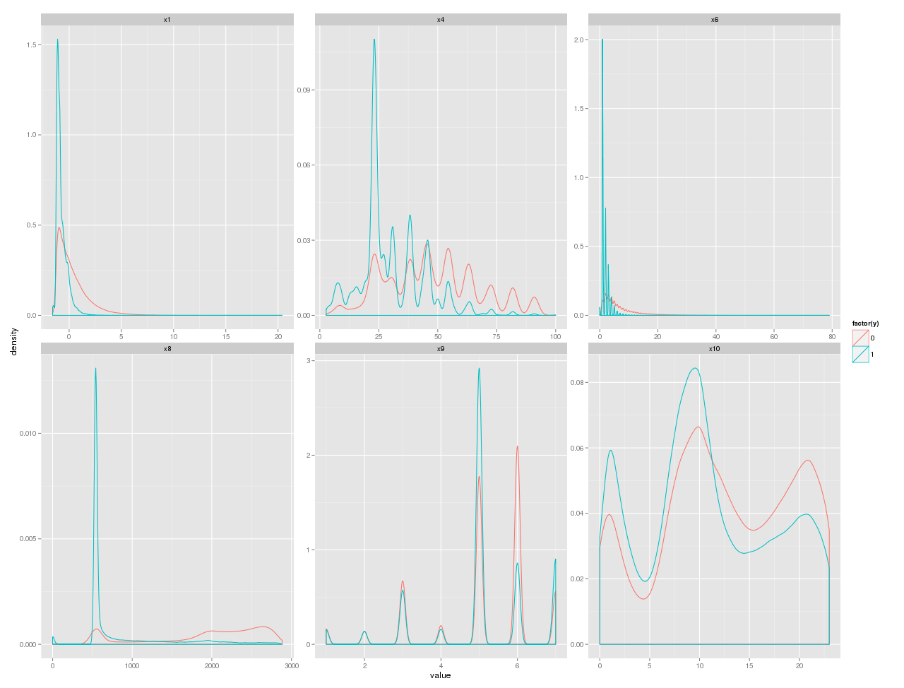
м—¬кё°м—җм„ңлҠ” к·ёлҰјмқ„ ліҙкі x6, x8мқҙ м„ нғқлҗҳм—ҲлӢӨ.
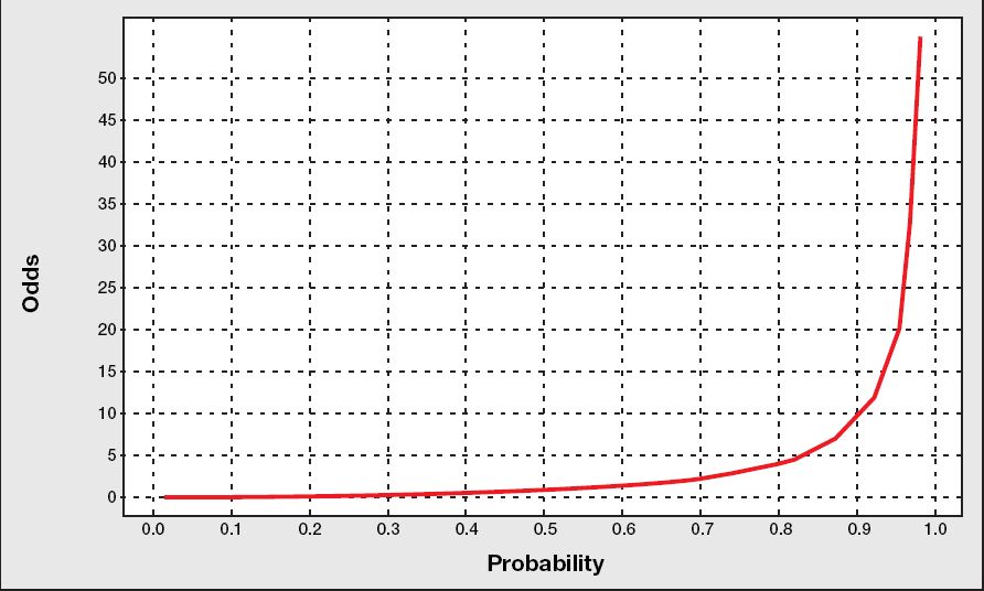
5 oddsмҷҖ logit #
мҠ№мӮ°(к·ёлҰј м¶ңмІҳ ->
м—¬кё°(http://www.bisolutions.us/Credit-Risk-Evaluation-of-Online-Personal-Loan-Applicants-A-Data-Mining-Approach.php))
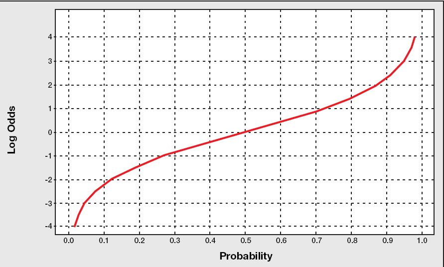
лЎң짓(к·ёлҰј м¶ңмІҳ ->
м—¬кё°(http://www.bisolutions.us/Credit-Risk-Evaluation-of-Online-Personal-Loan-Applicants-A-Data-Mining-Approach.php)) = logмҷҖ oddsлҘј н•©м№ңл§җ = log(1/(1-p))
pred <- predict(german.object, german, type="response")
logodds <- predict(german.object, german)
german <- cbind(german, pred) #нҷ•лҘ
german <- cbind(german, logodds) #мҳӨмҰҲ, odds
head(german)
кІ°кіј
> head(german)
   x1 x2  x3 x4 x5 x6 y       pred    logodds
1 A11  6 A34  4 67  1 0 0.18091034 -1.5101920
2 A12 48 A32  2 22  1 1 0.63503244  0.5538676
3 A14 12 A34  3 49  2 0 0.04865313 -2.9731627
4 A11 42 A32  4 45  2 0 0.64246423  0.5860757
5 A11 24 A33  4 53  2 1 0.46964395 -0.1215737
6 A14 36 A32  4 35  2 0 0.19922819 -1.3911252
2лІҲм§ё RowлҠ”
| x1 | x2 | x3 | x4 | x5 | x6 | y |
| A12 | 48 | A32 | 2 | 22 | 1 | 1 |
мқҙкі , нҡҢк·ҖмӢқмқҙ лӢӨмқҢкіј к°ҷмңјлҜҖлЎң
Coefficients:
             Estimate Std. Error z value Pr(>|z|)
(Intercept)  0.665099   0.476311   1.396 0.162607
x1A12       -0.531864   0.185402  -2.869 0.004121 **
x1A13       -1.076082   0.336956  -3.194 0.001405 **
x1A14       -1.898800   0.206314  -9.203  < 2e-16 ***
x2           0.034342   0.006329   5.426 5.76e-08 ***
x3A31       -0.099153   0.474942  -0.209 0.834629
x3A32       -0.946961   0.370644  -2.555 0.010622 *
x3A33       -0.934327   0.433303  -2.156 0.031061 *
x3A34       -1.526069   0.393754  -3.876 0.000106 ***
x5          -0.012765   0.007091  -1.800 0.071821 .
лӢӨмқҢкіј к°ҷмқҙ кі„мӮ°лҗңлӢӨ.
0.665099 -0.531864 + 48 * 0.034342 - 0.946961 -0.012765 * 22 = 0.5538676
нҷ•лҘ мқҖ..
x <- 0.665099 -0.531864 + 48 * 0.034342 - 0.946961 -0.012765 * 22
1 / (1 + exp(-x)) #кІ°кіјк°’ 0.6350307
exp(x) / (1 + exp(x)) #кІ°кіјк°’ 0.6350307, мқҙкІҢ лЎңм§ҖмҠӨнӢұ лӘЁнҳ•
кіј к°ҷмқҙ кі„мӮ°н•ҳл©ҙ лҗңлӢӨ.
8 분лҘҳн‘ң(confusion matrix) #
#T1 <- length(german[german$y==1 & german$pred > 0.5,]$x1)
#T0 <- length(german[german$y==0 & german$pred > 0.5,]$x1)
#F1 <- length(german[german$y==1 & german$pred <= 0.5,]$x1)
#F0 <- length(german[german$y==0 & german$pred <= 0.5,]$x1)
#
install.packages("SDMTools")
library("SDMTools")
confusion.matrix(german$y,german$pred,threshold=0.5)
кІ°кіј
> confusion.matrix(german$y,german$pred,threshold=0.5)
    obs
pred   0   1
   0 629 177
   1  71 123
attr(,"class")
[1] "confusion.matrix"
| | False(мӢӨм ң) | True(мӢӨм ң) |
| False(мҳҲмёЎ) | 629 | 177 |
| True(мҳҲмёЎ) | 71 | 123 |
| н•ӯлӘ© | кі„мӮ° | нҷ•лҘ (%) |
| м •нҷ•лҸ„ (Accuracy) | (629 + 123) / (629 + 177 + 71 + 123) | 75.20% |
| лҜјк°җлҸ„ (sensitivity) | 123 / (177 + 123) | 41.00% |
| нҠ№мқҙлҸ„ (specificity) | 629 / (629 + 71) | 89.86% |
| мҳӨлҘҳмңЁ (error) | (177 + 71 ) / (629 + 177 + 71 + 123) | 24.80% |
лӢӨмқҢкіј к°ҷмқҙ RлЎң кі„мӮ°н•ҙлҸ„ лҗңлӢӨ.
library("SDMTools")
mat <- confusion.matrix(german$y,german$pred,threshold=0.5)
mat
omission(mat)
sensitivity(mat)
specificity(mat)
prop.correct(mat)
кІ°кіј
> mat
    obs
pred   0   1
   0 629 177
   1  71 123
attr(,"class")
[1] "confusion.matrix"
> omission(mat)
[1] 0.59
> sensitivity(mat)
[1] 0.41
> specificity(mat)
[1] 0.8985714
> prop.correct(mat)
[1] 0.752
>
лӢӨмқҢкіј к°ҷмқҙ н•ҳл©ҙ лӢӨ лӮҳмҳЁлӢӨ.
> accuracy(german$y,german$pred,threshold=0.5)
  threshold       AUC omission.rate sensitivity specificity prop.correct     Kappa
1       0.5 0.6542857          0.59        0.41   0.8985714        0.752 0.3432203
>
к°’м—җ лҢҖн•ң м„ӨлӘ…
- AUC(area under curve): ROC curve м•„лһҳмқҳ л©ҙм Ғ, мҲ«мһҗк°Җ лҶ’мқ„мҲҳлЎқ мўӢлӢӨ.
- omission.rate: the ommission rate as a proportion of true occurrences misidentified given the defined threshold value
- sensitivity: 1мқј нҷ•лҘ , лҜјк°җлҸ„
- specificity: 0мқј нҷ•лҘ , нҠ№мқҙлҸ„
- prop.correct: лӘЁлҚёмқҳ м •нҷ•лҸ„
- kappa statistic
- Fleissмқҳ нҢҗлӢЁкё°мӨҖ..
- мӢ лў°лҸ„ лӮ®лӢӨ: 0.4 лҜёл§Ң
- мӢ лў°лҸ„ мһҲлӢӨ: 0.4 ~ 0.6
- мӢ лў°лҸ„ лҶ’лӢӨ: 0.6 ~ 0.75
- мӢ лў°лҸ„ л§Өмҡ° лҶ’лӢӨ: 0.75 мҙҲкіј
м°ёкі : мөңм Ғ(м •нҷ•лҸ„)мқҳ threshold м°ҫкё°
for (i in seq(0,1,0.01))
{
  rs <- c(rs, accuracy(x2$t0,x2$pred,threshold=i)$prop.correct)
}

max_val = max(rs)
for (i in seq(0,1,0.01))
{
  tmp <- accuracy(x2$t0,x2$pred,threshold=i)$prop.correct
  if ( max_val == tmp )
  {
    print (paste("threshold = ", i))
  }
}
9 ROC(Receiver-Operating Characteristic curve) кіЎм„ #
install.packages("ROCR")
library("ROCR")
cname <- c("x1", "x2", "x3","x4", "x5", "x6", "y")
german = read.table("c:\\data\\german1.txt", col.names = cname)
options(contrasts = c("contr.treatment", "contr.poly"))
german.object <- glm(formula = y ~ x1 + x2 + x3 + x5, family = binomial, data = german)
pred <- predict(german.object, german, type="response")
logodds <- predict(german.object, german)
german <- cbind(german, pred)
german <- cbind(german, logodds)
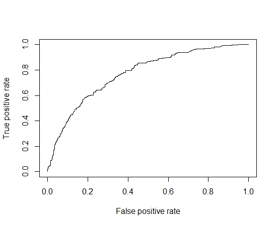
roc = prediction(german$pred, german$y)
perf = performance(roc, "tpr", "fpr")
#"tpr"мқҖ hit rate, "fpr"мқҖ н—ӣкІҪліҙмңЁ(false alarm rate)
plot(perf)
#plot(perf, print.cutoff.at=seq(0,1,by=0.1))
11 кІҖм • #
install.packages("logistf")
library("logistf")
lr2 = logistf(y ~ x1 + x2 + x3 + x5, data = german)
summary(lr2)
кІ°кіј
> summary(lr2)
logistf(formula = y ~ x1 + x2 + x3 + x5, data = german)

Model fitted by Penalized ML
Confidence intervals and p-values by Profile Likelihood

                   coef    se(coef)  lower 0.95   upper 0.95       Chisq
(Intercept)  0.64472876 0.474759083 -0.27043182  1.581359116  1.89900357
x1A12       -0.52660853 0.185120846 -0.88988344 -0.166823398  8.25198090
x1A13       -1.04548754 0.334474867 -1.72559520 -0.417128337 11.03319913
x1A14       -1.87794257 0.205266409 -2.28709164 -1.483111213         Inf
x2           0.03387929 0.006308928  0.02165981  0.046313848 29.94733537
x3A31       -0.09194231 0.473477203 -1.01911361  0.824239056  0.03855106
x3A32       -0.92696865 0.369386547 -1.66277580 -0.221680910  6.67102543
x3A33       -0.90779881 0.431809628 -1.76384501 -0.081117723  4.64170188
x3A34       -1.49870282 0.392307541 -2.27839153 -0.748208241 15.50420478
x5          -0.01252255 0.007063063 -0.02651766  0.001115517  3.23324577
                       p
(Intercept) 1.681899e-01
x1A12       4.070755e-03
x1A13       8.949457e-04
x1A14       0.000000e+00
x2          4.439416e-08
x3A31       8.443407e-01
x3A32       9.799279e-03
x3A33       3.120404e-02
x3A34       8.232193e-05
x5          7.215754e-02

Likelihood ratio test=200.5529 on 9 df, p=0, n=1000
Wald test = 152.8214 on 9 df, p = 0

Covariance-Matrix:
              [,1]          [,2]          [,3]          [,4]          [,5]
 [1,]  0.225396187 -2.116841e-02 -0.0178520944 -1.475598e-02 -1.030299e-03
 [2,] -0.021168410  3.426973e-02  0.0158947775  1.663656e-02 -4.993463e-05
 [3,] -0.017852094  1.589478e-02  0.1118734364  1.582290e-02  1.008258e-04
 [4,] -0.014755985  1.663656e-02  0.0158228986  4.213430e-02 -6.926150e-05
 [5,] -0.001030299 -4.993463e-05  0.0001008258 -6.926150e-05  3.980257e-05
 [6,] -0.129133562  4.653294e-03  0.0017777035  2.271459e-03  1.822720e-04
 [7,] -0.134642541  3.932850e-03  0.0010335670  1.458292e-04  2.134383e-04
 [8,] -0.118628622 -2.470301e-03  0.0005935660 -5.484439e-03 -2.417103e-05
 [9,] -0.126861265  4.418244e-03  0.0018526164 -2.134237e-03  2.052452e-04
[10,] -0.001743630  7.292805e-05 -0.0000437410  1.938701e-05 -1.300694e-07
               [,6]          [,7]          [,8]          [,9]         [,10]
 [1,] -1.291336e-01 -1.346425e-01 -1.186286e-01 -0.1268612649 -1.743630e-03
 [2,]  4.653294e-03  3.932850e-03 -2.470301e-03  0.0044182436  7.292805e-05
 [3,]  1.777704e-03  1.033567e-03  5.935660e-04  0.0018526164 -4.374100e-05
 [4,]  2.271459e-03  1.458292e-04 -5.484439e-03 -0.0021342366  1.938701e-05
 [5,]  1.822720e-04  2.134383e-04 -2.417103e-05  0.0002052452 -1.300694e-07
 [6,]  2.241807e-01  1.258971e-01  1.240776e-01  0.1263132224 -8.388392e-05
 [7,]  1.258971e-01  1.364464e-01  1.240557e-01  0.1260949748  7.408724e-05
 [8,]  1.240776e-01  1.240557e-01  1.864596e-01  0.1247551153 -9.031551e-05
 [9,]  1.263132e-01  1.260950e-01  1.247551e-01  0.1539052064 -1.431441e-04
[10,] -8.388392e-05  7.408724e-05 -9.031551e-05 -0.0001431441  4.988686e-05
мқҙлҹ°кұ°лҸ„ мһҲлӢӨ.
install.packages("survey")
library("survey")
regTermTest(german.object, ~x1 + x2 + x3 + x5)
кІ°кіј
> regTermTest(german.object, ~x1 + x2 + x3 + x5)
Wald test for x1 x2 x3 x5
 in glm(formula = y ~ x1 + x2 + x3 + x5, family = binomial, data = german)
F =  17.2046  on  9  and  990  df: p= < 2.22e-16
p-valueк°Җ мЎ°л„Ё мһ‘мңјлӢҲк№Ң к·Җл¬ҙк°Җм„Ө м§Җм§Җ лӘ»н•Ё. мҰү, м°Ёмқҙк°Җ мһҲмқҢ.
 german1.txt) нҷңмҡ©