[edit]
5 n개의 집단 비율에 대한 검정 #
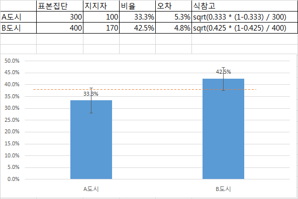
A도시에서는 300명 중 100명이, B도시에서는 400명 중 170명이 D후보를 지지한다고 조사되었다. A도시와 B도시의 D후부 지지 비율이 같다고 할 수 있는가?
분자 <- c(100, 170)
분모 <- c(300, 400)
prop.test(분자, 분모)
> prop.test(분자, 분모)

	2-sample test for equality of proportions with continuity correction

data:  분자 out of 분모
X-squared = 5.6988, df = 1, p-value = 0.01698
alternative hypothesis: two.sided
95 percent confidence interval:
 -0.16664176 -0.01669158
sample estimates:
   prop 1    prop 2
0.3333333 0.4250000
결과해석
- 두 집단에서 어떤 사건에 대한 비율이 같다고 할 수 있는지에 대한 검정.
- 가설
- 귀무가설: 차이가 없다.
- 대립가설: 차이가 있다. --> 유의수준 0.05에서는 대립가설 지지, 유의수준 0.01에서는 대립가설 기각
- 귀무가설: 차이가 없다.
- 95% 신뢰구간: 0.4250000-0.16664176 ~ 0.4250000-0.01669158 = 0.2583582 ~ 0.4083084, 기준은 100/300