[edit]
1 SE, Standard Error #
лӘҪл‘Ҙмқҳ кёёмқҙлҘј 5нҡҢ мёЎм •н–ҲлӢӨ.
x <- c(76.2, 76.3, 76.1, 76,3, 76.4)
se <- sd(x)/sqrt(length(x)) #0.6009252
se #1.643168
н•ҷмғқ 2,000лӘ…мқҳ мҲҳн•ҷ лӘЁмқҳкі мӮ¬ м„ұм Ғмқҙ мһҲлӢӨ.
set.seed(1000) x <- rnorm(2000, mean = 70, sd = 10) summary(x)кІ°кіј
> summary(x)
   Min. 1st Qu.  Median    Mean 3rd Qu.    Max.
  36.38   63.33   69.89   69.94   76.54   99.19
н‘ңмӨҖмҳӨм°ЁлҠ”..
mu <- c()
for(i in 1:100){
    mu <- c(mean(sample(x, 5)), mu)
}

se <- sd(mu) / sqrt(5)
mean(mu) #69.82971
se #1.935552
[edit]
2 нҸүк· мқ„ 비көҗн•ҳлҠ” кІҖм • л°©лІ• #
| м •к·ң분нҸ¬ м—¬л¶Җ | кІҖм •лІ• |
| Y | t кІҖм •, 분мӮ°л¶„м„қ |
| N | Wilcoxon кІҖм •, Kurskal-Wallis кІҖм • |
- Two-sample t-test <-> Wilcoxonrank sum test
- Paired t-test <-> Wilcoxonsigned rank test
[edit]
3 t кІҖм • к°ңмҡ” #
- нҸүк· мқ„ 비көҗн•ҳм—¬ н•ҙлӢ№ 집лӢЁмқҳ лҢҖн‘ңк°’мңјлЎңмқҳ м—ӯн• мқ„ н•ҳкі мһҲлӢӨлҠ” кІғмқ„ мқҳлҜён•Ё.
- мқҙмғҒм№ҳ(outlier)к°Җ мһҲлҠ” м •к·ң분нҸ¬к°Җ м•„лӢҢ лҚ°мқҙн„°лҠ” t кІҖм • н•ҳл©ҙ м•ҲлҗЁ.
- м •к·ң분нҸ¬м—¬л¶Җ нҷ•мқё н•ҳлҠ” л°©лІ•
- мқҙмғҒм№ҳ м ңкұ° л°©лІ•
[edit]
4 One Sample t-test #
2н•ҷл…„ 1л°ҳмқҳ 2011л…„ н•ҳлЈЁ нҸүк· кІҢмһ„мӢңк°„ 2.1мӢңк°„ мқҙм—ҲлӢӨ. 2012л…„м—җ 10лӘ…мқ„ л¬ҙмһ‘мң„лЎң м„ л°ңн•ҳм—¬ кІҢмһ„ мӢңк°„мқ„ мЎ°мӮ¬н•ҳмҳҖлӢӨ. 2011л…„кіј 2012л…„мқҙ лӢӨлҘёк°Җ?
x <- c(3.3, 2.8, 3.0, 2.7, 2.7, 2.0, 1.9, 3.4, 1.4, 1.4)
t.test(x, mu=2.1)
м •к·ңм„ұ кІҖм •
> shapiro.test(x)

	Shapiro-Wilk normality test

data:  x
W = 0.9085, p-value = 0.2711
- к°Җм„Ө
- к·Җл¬ҙк°Җм„Ө: м •к·ң분нҸ¬мҷҖ м°Ёмқҙк°Җ м—ҶлӢӨ.
- лҢҖлҰҪк°Җм„Ө: м •к·ң분нҸ¬мҷҖ м°Ёмқҙк°Җ мһҲлӢӨ.
- к·Җл¬ҙк°Җм„Ө: м •к·ң분нҸ¬мҷҖ м°Ёмқҙк°Җ м—ҶлӢӨ.
- мң мқҳмҲҳмӨҖ 0.05лқјкі н–Ҳмқ„ л•Ң, p-valueк°Җ 0.2711мқҙлҜҖлЎң к·Җл¬ҙк°Җм„Ө кё°к°Ғн•ҳм§Җ лӘ»н•Ё. мҰү, м •к·ң분нҸ¬лӢӨ.
> t.test(x, mu=2.1)

	One Sample t-test

data:  x
t = 1.5454, df = 9, p-value = 0.1567
alternative hypothesis: true mean is not equal to 2.1
95 percent confidence interval:
 1.933026 2.986974
sample estimates:
mean of x
     2.46
- к°Җм„Ө
- к·Җл¬ҙк°Җм„Ө: нҸүк· м—җ м°Ёмқҙк°Җ м—ҶлӢӨ.
- лҢҖлҰҪк°Җм„Ө: нҸүк· м—җ м°Ёмқҙк°Җ мһҲлӢӨ.
- к·Җл¬ҙк°Җм„Ө: нҸүк· м—җ м°Ёмқҙк°Җ м—ҶлӢӨ.
- мң мқҳмҲҳмӨҖ 0.05лқјкі н–Ҳмқ„ л•Ң, p-valueк°Җ 0.1567мқҙлҜҖлЎң к·Җл¬ҙк°Җм„Ө кё°к°Ғн•ҳм§Җ лӘ»н•Ё.
> t.test(x)

	One Sample t-test

data:  x
t = 10.6, df = 9, p-value = 2.269e-06
alternative hypothesis: true mean is not equal to 0
95 percent confidence interval:
 1.93 2.99
sample estimates:
mean of x
     2.46
[edit]
5 Two Sample t-test #
- л‘җ 집лӢЁмқҳ нҸүк· л№„көҗ
- к°Җм •
- л‘җ 집лӢЁмқҙ м •к·ң분нҸ¬
- л‘җ 집лӢЁмқҙ 분мӮ°мқҙ к°ҷмқҢ
- л‘җ 집лӢЁмқҙ м •к·ң분нҸ¬
x1 <- c(15,10,13,7,9,8,21,9,14,8)
x2 <- c(15,14,12,8,14,7,16,10,15,12)
м •к·ңм„ұ кІҖм • --> x1, x2к°Җ мң мқҳмҲҳмӨҖ 0.05м—җм„ң м •к·ң분нҸ¬мһ„.
> shapiro.test(x1)

	Shapiro-Wilk normality test

data:  x1
W = 0.8666, p-value = 0.09131

> shapiro.test(x2)

	Shapiro-Wilk normality test

data:  x2
W = 0.9125, p-value = 0.2986
분мӮ°мқҙ лҸҷмқјн•ңк°Җ?
> var.test(x1, x2)

	F test to compare two variances

data:  x1 and x2
F = 1.9791, num df = 9, denom df = 9, p-value = 0.3237
alternative hypothesis: true ratio of variances is not equal to 1
95 percent confidence interval:
 0.491579 7.967821
sample estimates:
ratio of variances
          1.979094
- к°Җм„Ө
- к·Җл¬ҙк°Җм„Ө: x1кіј x2лҠ” 분мӮ°мқҳ м°Ёмқҙк°Җ м—ҶлӢӨ.
- лҢҖлҰҪк°Җм„Ө: x1кіј x2лҠ” 분мӮ°мқҳ м°Ёмқҙк°Җ мһҲлӢӨ.
- к·Җл¬ҙк°Җм„Ө: x1кіј x2лҠ” 분мӮ°мқҳ м°Ёмқҙк°Җ м—ҶлӢӨ.
- мң мқҳмҲҳмӨҖ 0.05лқјкі н–Ҳмқ„ л•Ң, p-valueк°Җ 0.3237мқҙлҜҖлЎң к·Җл¬ҙк°Җм„Ө кё°к°Ғн•ҳм§Җ лӘ»н•Ё. мҰү, 분мӮ°мқҳ м°Ёмқҙк°Җ м—ҶлӢӨ.
> t.test(x1, x2, var.equal=T)

	Two Sample t-test

data:  x1 and x2
t = -0.5331, df = 18, p-value = 0.6005
alternative hypothesis: true difference in means is not equal to 0
95 percent confidence interval:
 -4.446765  2.646765
sample estimates:
mean of x mean of y
     11.4      12.3
- к°Җм„Ө
- к·Җл¬ҙк°Җм„Ө: x1кіј x2лҠ” нҸүк· мқҳ м°Ёмқҙк°Җ м—ҶлӢӨ.
- лҢҖлҰҪк°Җм„Ө: x1кіј x2лҠ” нҸүк· мқҳ м°Ёмқҙк°Җ мһҲлӢӨ.
- к·Җл¬ҙк°Җм„Ө: x1кіј x2лҠ” нҸүк· мқҳ м°Ёмқҙк°Җ м—ҶлӢӨ.
- мң мқҳмҲҳмӨҖ 0.05лқјкі н–Ҳмқ„ л•Ң, p-valueк°Җ 0.6005мқҙлҜҖлЎң к·Җл¬ҙк°Җм„Ө кё°к°Ғн•ҳм§Җ лӘ»н•Ё. мҰү, л‘җ 집лӢЁк°„ нҸүк· мқҳ м°Ёмқҙк°Җ м—ҶлӢӨ.
> t.test(x1, x2, alternative="less", var.equal=T)

	Two Sample t-test

data:  x1 and x2
t = -0.5331, df = 18, p-value = 0.3002
alternative hypothesis: true difference in means is less than 0
95 percent confidence interval:
     -Inf 2.027436
sample estimates:
mean of x mean of y
     11.4      12.3
[edit]
6 Paired t-test #
- Paired -> 11мӣ”м—җ 30лӘ…мқ„ 추м¶ңн•ҳм—¬ лӘёл¬ҙкІҢлҘј мёЎм •н–Ҳкі , 12мӣ”м—җ 11мӣ”м—җ 추м¶ңлҗң 30лӘ…мқҳ лӘёл¬ҙкІҢлҘј лӢӨмӢң мёЎм •н•ҳм—¬ нҸүк· м°Ёмқҙк°Җ мһҲлҠ”м§Җ кІҖм • н• л•Ң..
- лӮҳлЁём§ҖлҠ” Two Sample t-testмҷҖ лҸҷмқј
- Two Sample t-test мҳҲм ңм—җм„ңмқҳ лҚ°мқҙн„°к°Җ Paired лҚ°мқҙн„°лқјл©ҙ..
> t.test(x1, x2, var.equal=T, paired=T)

	Paired t-test

data:  x1 and x2
t = -0.9612, df = 9, p-value = 0.3616
alternative hypothesis: true difference in means is not equal to 0
95 percent confidence interval:
 -3.018069  1.218069
sample estimates:
mean of the differences
                   -0.9
- к°Җм„Ө
- к·Җл¬ҙк°Җм„Ө: x1кіј x2лҠ” нҸүк· мқҳ м°Ёмқҙк°Җ м—ҶлӢӨ.
- лҢҖлҰҪк°Җм„Ө: x1кіј x2лҠ” нҸүк· мқҳ м°Ёмқҙк°Җ мһҲлӢӨ.
- к·Җл¬ҙк°Җм„Ө: x1кіј x2лҠ” нҸүк· мқҳ м°Ёмқҙк°Җ м—ҶлӢӨ.
- мң мқҳмҲҳмӨҖ 0.05лқјкі н–Ҳмқ„ л•Ң, p-valueк°Җ 0.3616мқҙлҜҖлЎң к·Җл¬ҙк°Җм„Ө кё°к°Ғн•ҳм§Җ лӘ»н•Ё. мҰү, л‘җ 집лӢЁк°„ нҸүк· мқҳ м°Ёмқҙк°Җ м—ҶлӢӨ.
[edit]
7 분мӮ°л¶„м„қ #
- 3к°ң мқҙмғҒмқҳ 집лӢЁм—җ лҢҖн•ң нҸүк· мқҳ м°Ёмқҙ кІҖм •(two-sample testмқҳ нҷ•мһҘ)
- 분мӮ°л¶„м„қ
- мқјмӣҗ분мӮ°л¶„м„қ(one-way ANOVA) - 1к°ңмқҳ к·ёлЈ№ліҖмҲҳ
- мқҙмӣҗ분мӮ°л¶„м„қ(two-way ANOVA) - 2к°ңмқҳ к·ёлЈ№ліҖмҲҳ
- кіө분мӮ°л¶„м„қ(ANCOVA; Analysis of Covariance) - мқјмӣҗ분мӮ°л¶„м„қм—җ м—°мҶҚнҳ• ліҖмҲҳ кіөліҖлҹү(covariate)추к°Җ
- мқјмӣҗ분мӮ°л¶„м„қ(one-way ANOVA) - 1к°ңмқҳ к·ёлЈ№ліҖмҲҳ
- кё°ліём Ғмқё к°Җм •
- 집лӢЁк°„ лҸ…лҰҪ
- м •к·ң분нҸ¬лҘј л”°лқјм•ј н•Ё
- лҸҷмқјн•ң 분мӮ°
- 집лӢЁк°„ лҸ…лҰҪ
- кё°ліём Ғмқё к°Җм •м—җ л§һм§Җ м•ҠлҠ” кІҪмҡ°
- 분мӮ°л¶„м„қ лҢҖмӢ Kurskal-Wallis Test
- 분мӮ°л¶„м„қ лҢҖмӢ Kurskal-Wallis Test
[edit]
8 мқјмӣҗ분мӮ°л¶„м„қ #
#http://code.google.com/p/sonya/source/browse/trunk/r-project/sample/PlantGrowth.csv
plantGrowth = read.csv("c:\\data\\PlantGrowth.csv")
head(plantGrowth)
boxplot(weight ~ group, data=plantGrowth)
out <- lm(weight ~ group, data=plantGrowth)
summary(out)
anova(out)
> summary(out)
Call:
lm(formula = weight ~ group, data = plantGrowth)
Residuals:
Min 1Q Median 3Q Max
-1.0710 -0.4180 -0.0060 0.2627 1.3690
Coefficients:
Estimate Std. Error t value Pr(>|t|)
(Intercept) 5.0320 0.1971 25.527 <2e-16 ***
grouptrt1 -0.3710 0.2788 -1.331 0.1944
grouptrt2 0.4940 0.2788 1.772 0.0877 .
---
Signif. codes: 0 вҖҳ***вҖҷ 0.001 вҖҳ**вҖҷ 0.01 вҖҳ*вҖҷ 0.05 вҖҳ.вҖҷ 0.1 вҖҳ вҖҷ 1
Residual standard error: 0.6234 on 27 degrees of freedom
Multiple R-squared: 0.2641, Adjusted R-squared: 0.2096
F-statistic: 4.846 on 2 and 27 DF, p-value: 0.01591
> anova(out)
Analysis of Variance Table
Response: weight
Df Sum Sq Mean Sq F value Pr(>F)
group 2 3.7663 1.8832 4.8461 0.01591 *
Residuals 27 10.4921 0.3886
---
Signif. codes: 0 вҖҳ***вҖҷ 0.001 вҖҳ**вҖҷ 0.01 вҖҳ*вҖҷ 0.05 вҖҳ.вҖҷ 0.1 вҖҳ вҖҷ 1
- к°Җм„Ө
- к·Җл¬ҙк°Җм„Ө: 3к·ёлЈ№мқҳ нҸүк· мқҙ к°ҷлӢӨ.
- лҢҖлҰҪк°Җм„Ө: 3к·ёлЈ№мқҳ нҸүк· мқҙ лӢӨлҘҙлӢӨ.
- к·Җл¬ҙк°Җм„Ө: 3к·ёлЈ№мқҳ нҸүк· мқҙ к°ҷлӢӨ.
- мң мқҳмҲҳмӨҖ 0.05лқјкі н–Ҳмқ„ л•Ң, p-valueк°Җ 0.01591мқҙлҜҖлЎң к·Җл¬ҙк°Җм„Ө кё°к°Ғ. мҰү, 3к·ёлЈ№мқҙ нҸүк· мқҳ м°Ёмқҙк°Җ мһҲлӢӨ.
- к·ёлҹ¬лӮҳ, нҡҢк·Җ진лӢЁмқ„ н•ҙлҙҗм•ј м Ғн•©н•ңм§Җ м•Ң мҲҳ мһҲмқҢ.
par(mfrow=c(2,2))
plot(out)
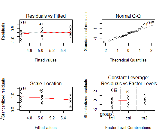
м •к·ңм„ұ -> p-value = 0.4379мқҙлҜҖлЎң м •к·ң분нҸ¬лӢӨ.
> shapiro.test(resid(out))

	Shapiro-Wilk normality test

data:  resid(out)
W = 0.9661, p-value = 0.4379
л“ұ분мӮ°м„ұ -> p-value = 0.1714лЎң к·Җл¬ҙк°Җм„Ө м§Җм§Җ. мҰү, л“ұ분мӮ°
#library("lmtest")
> bptest(out)

	studentized Breusch-Pagan test

data:  out
BP = 3.5273, df = 2, p-value = 0.1714
лҸ…лҰҪм„ұ
> dwtest(out) #library("lmtest")

	Durbin-Watson test

data:  out
DW = 2.704, p-value = 0.9502
alternative hypothesis: true autocorrelation is greater than 0
- dнҶөкі„лҹү
- 0 : м–‘мқҳ мһҗкё°мғҒкҙҖ, p-value = 1
- 2 : лҸ…лҰҪ, p-value = 0
- 4 : мқҢмқҳ мһҗкё°мғҒкҙҖ, p-value = -1
- 0 : м–‘мқҳ мһҗкё°мғҒкҙҖ, p-value = 1
- лҢҖлһөм ҒмңјлЎң DWк°’мқҙ 1ліҙлӢӨ мһ‘кұ°лӮҳ 3ліҙлӢӨ нҒ¬л©ҙ мһҗкё°мғҒкҙҖмқҙ нҷ•мӢӨнһҲ мһҲлӢӨкі нҢҗлӢ¬н• мҲҳ мһҲмңјл©°, 1.5~2.5 мӮ¬мқҙм—җ мһҲмқ„ кІҪмҡ° лҸ…лҰҪмқҙлқјкі нҢҗлӢЁ
- лҢҖлһө лҸ…лҰҪ.
л°©лІ•1: Dunnett -> нҸүк· мқҳ м°Ёмқҙк°Җ м—ҶлҠ” мЎ°н•©мқ„ ліҙм—¬мӨҖлӢӨ. (control лҢҖ비 비көҗлІ•)
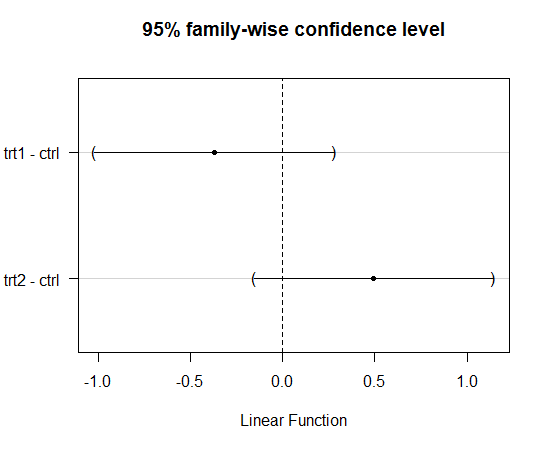
95% мӢ лў°кө¬к°„мқҙ 0мқ„ нҸ¬н•Ё
install.packages("multcomp")
library("multcomp")
out <- lm(weight ~ group, data=PlantGrowth)
dunnett <- glht(out, linfct=mcp(group="Dunnett")) #м—¬кё°м„ң groupмқҖ plantGrowth$group мқҙлӢӨ.
summary(dunnett)
plot(dunnett)
95% мӢ лў°кө¬к°„мқҙ 0мқ„ нҸ¬н•Ё
> summary(dunnett)

	 Simultaneous Tests for General Linear Hypotheses

Multiple Comparisons of Means: Dunnett Contrasts


Fit: lm(formula = weight ~ group, data = PlantGrowth)

Linear Hypotheses:
                 Estimate Std. Error t value Pr(>|t|)
trt1 - ctrl == 0  -0.3710     0.2788  -1.331    0.323
trt2 - ctrl == 0   0.4940     0.2788   1.772    0.153
(Adjusted p values reported -- single-step method)
- trt1 - ctrlмқҳ p-value = 0.323 -> к·Җл¬ҙк°Җм„Ө м§Җм§Җ, нҸүк· мқҳ м°Ёмқҙ м—ҶмқҢ
- trt2 - ctrlмқҳ p-value = 0.153 -> к·Җл¬ҙк°Җм„Ө м§Җм§Җ, нҸүк· мқҳ м°Ёмқҙ м—ҶмқҢ
install.packages("multcomp")
library("multcomp")
out <- lm(weight ~ group, data=PlantGrowth)
tukey <- glht(out, linfct=mcp(group="Tukey")) #м—¬кё°м„ң groupмқҖ PlantGrowth$group мқҙлӢӨ.
summary(tukey)
plot(tukey)
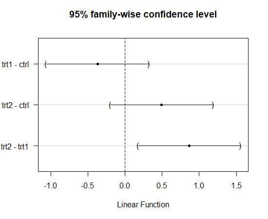
> summary(tukey)
Simultaneous Tests for General Linear Hypotheses
Multiple Comparisons of Means: Tukey Contrasts
Fit: lm(formula = weight ~ group, data = plantGrowth)
Linear Hypotheses:
Estimate Std. Error t value Pr(>|t|)
trt1 - ctrl == 0 -0.3710 0.2788 -1.331 0.391
trt2 - ctrl == 0 0.4940 0.2788 1.772 0.198
trt2 - trt1 == 0 0.8650 0.2788 3.103 0.012 *
---
Signif. codes: 0 вҖҳ***вҖҷ 0.001 вҖҳ**вҖҷ 0.01 вҖҳ*вҖҷ 0.05 вҖҳ.вҖҷ 0.1 вҖҳ вҖҷ 1
(Adjusted p values reported -- single-step method)
- trt1 - ctrlмқҳ p-value = 0.323 -> к·Җл¬ҙк°Җм„Ө м§Җм§Җ, нҸүк· мқҳ м°Ёмқҙ м—ҶмқҢ
- trt2 - ctrlмқҳ p-value = 0.153 -> к·Җл¬ҙк°Җм„Ө м§Җм§Җ, нҸүк· мқҳ м°Ёмқҙ м—ҶмқҢ
- trt2 - trt1мқҳ p-value = 0.153 -> к·Җл¬ҙк°Җм„Ө кё°к°Ғ, нҸүк· мқҳ м°Ёмқҙ мһҲмқҢ
[edit]
9 мқҙмӣҗ분мӮ°л¶„м„қ #
#http://code.google.com/p/sonya/source/browse/trunk/r-project/sample/warpbreaks.csv?r=653
warpbreaks = read.csv("c:\\data\\warpbreaks.csv")
мқҙмӮ°нҳ• ліҖмҲҳмқё woolкіј tensionмқҳ мҲңм„ң нҷ•мқё
> levels(warpbreaks$wool)
[1] "A" "B"
> levels(warpbreaks$tension)
[1] "L" "M" "H"
- wool -> мҲңм„ңк°Җ л§һмқҢ.
- tension -> мҲңм„ңк°Җ л§һм§Җ м•ҠмқҢ. L, M, H мҲңм„ңмқҙм–ҙм•ј н•Ё.
> warpbreaks$tension = factor(warpbreaks$tension, level = c("L", "M", "H"))
> levels(warpbreaks$tension)
[1] "L" "M" "H"
분мӮ°л¶„м„қ
out <- lm(breaks ~ wool*tension, data = warpbreaks)
summary(out)
> summary(out)
Call:
lm(formula = breaks ~ wool * tension, data = warpbreaks)
Residuals:
Min 1Q Median 3Q Max
-19.5556 -6.8889 -0.6667 7.1944 25.4444
Coefficients:
Estimate Std. Error t value Pr(>|t|)
(Intercept) 44.556 3.647 12.218 2.43e-16 ***
woolB -16.333 5.157 -3.167 0.002677 **
tensionM -20.556 5.157 -3.986 0.000228 ***
tensionH -20.000 5.157 -3.878 0.000320 ***
woolB:tensionM 21.111 7.294 2.895 0.005698 **
woolB:tensionH 10.556 7.294 1.447 0.154327
---
Signif. codes: 0 вҖҳ***вҖҷ 0.001 вҖҳ**вҖҷ 0.01 вҖҳ*вҖҷ 0.05 вҖҳ.вҖҷ 0.1 вҖҳ вҖҷ 1
Residual standard error: 10.94 on 48 degrees of freedom
Multiple R-squared: 0.3778, Adjusted R-squared: 0.3129
F-statistic: 5.828 on 5 and 48 DF, p-value: 0.0002772
- нҸүк· м—җ м°Ёмқҙк°Җ мһҲмқҢ(м•„м§Ғ нҡҢк·Җ진лӢЁмқ„ н•ҳм§ҖлҠ” м•ҠмқҖ мғҒнғң)
- көҗнҳёмһ‘мҡ©мқҙ мһҲмқҢмқ„ нҷ•мқё
- woolB:tensionM -> p-value = 0.005698, мң мқҳмҲҳмӨҖ 0.05м—җм„ң к·Җл¬ҙк°Җм„Ө кё°к°Ғ => көҗнҳёмһ‘мҡ© нҷ•мқён•Ё!!
- woolB:tensionH -> p-value = 0.154327, мң мқҳмҲҳмӨҖ 0.05м—җм„ң к·Җл¬ҙк°Җм„Ө м§Җм§Җ
- woolB:tensionM -> p-value = 0.005698, мң мқҳмҲҳмӨҖ 0.05м—җм„ң к·Җл¬ҙк°Җм„Ө кё°к°Ғ => көҗнҳёмһ‘мҡ© нҷ•мқён•Ё!!
> shapiro.test(resid(out))

	Shapiro-Wilk normality test

data:  resid(out)
W = 0.9869, p-value = 0.8162
л“ұ분мӮ°м„ұ -> p-value = 0.0006307лЎң к·Җл¬ҙк°Җм„Ө кё°к°Ғ. мҰү, л“ұ분мӮ°мқҙ м•„лӢҳ. мў…мҶҚліҖмҲҳ breaksм—җ log()лӮҳ sqrt()н•ҳмһҗ.
#library("lmtest")
> bptest(out)

	studentized Breusch-Pagan test

data:  out
BP = 21.5744, df = 5, p-value = 0.0006307
лҸ…лҰҪм„ұ
> dwtest(out)

	Durbin-Watson test

data:  out
DW = 2.2376, p-value = 0.575
alternative hypothesis: true autocorrelation is greater than 0
- dнҶөкі„лҹү
- 0 : м–‘мқҳ мһҗкё°мғҒкҙҖ, p-value = 1
- 2 : лҸ…лҰҪ, p-value = 0
- 4 : мқҢмқҳ мһҗкё°мғҒкҙҖ, p-value = -1
- 0 : м–‘мқҳ мһҗкё°мғҒкҙҖ, p-value = 1
- лҢҖлһөм ҒмңјлЎң DWк°’мқҙ 1ліҙлӢӨ мһ‘кұ°лӮҳ 3ліҙлӢӨ нҒ¬л©ҙ мһҗкё°мғҒкҙҖмқҙ нҷ•мӢӨнһҲ мһҲлӢӨкі нҢҗлӢ¬н• мҲҳ мһҲмңјл©°, 1.5~2.5 мӮ¬мқҙм—җ мһҲмқ„ кІҪмҡ° лҸ…лҰҪмқҙлқјкі нҢҗлӢЁ
- лҢҖлһө лҸ…лҰҪ.
> out <- lm(log(breaks) ~ wool*tension, data = warpbreaks)
> shapiro.test(resid(out))

	Shapiro-Wilk normality test

data:  resid(out)
W = 0.9729, p-value = 0.2583

> bptest(out)

	studentized Breusch-Pagan test

data:  out
BP = 4.8045, df = 5, p-value = 0.4402

> dwtest(out)

	Durbin-Watson test

data:  out
DW = 2.06, p-value = 0.3167
alternative hypothesis: true autocorrelation is greater than 0
- м •к·ңм„ұ, л“ұ분мӮ°м„ұ, лҸ…лҰҪм„ұмқҙ лӘЁл‘җ к° м¶ҳн•Ё.
library("multcomp")
out <- lm(log(breaks) ~ wool + tension, data=warpbreaks)
tukey1 <- glht(out, linfct=mcp(wool="Tukey"))
tukey2 <- glht(out, linfct=mcp(tension="Tukey"))
summary(tukey1)
summary(tukey2)
> summary(tukey1)
Simultaneous Tests for General Linear Hypotheses
Multiple Comparisons of Means: Tukey Contrasts
Fit: lm(formula = log(breaks) ~ wool + tension, data = warpbreaks)
Linear Hypotheses:
Estimate Std. Error t value Pr(>|t|)
B - A == 0 -0.1522 0.1063 -1.431 0.159
(Adjusted p values reported -- single-step method)
> summary(tukey2)
Simultaneous Tests for General Linear Hypotheses
Multiple Comparisons of Means: Tukey Contrasts
Fit: lm(formula = log(breaks) ~ wool + tension, data = warpbreaks)
Linear Hypotheses:
Estimate Std. Error t value Pr(>|t|)
M - L == 0 -0.2871 0.1302 -2.205 0.08018 .
H - L == 0 -0.4893 0.1302 -3.758 0.00133 **
H - M == 0 -0.2022 0.1302 -1.553 0.27550
---
Signif. codes: 0 вҖҳ***вҖҷ 0.001 вҖҳ**вҖҷ 0.01 вҖҳ*вҖҷ 0.05 вҖҳ.вҖҷ 0.1 вҖҳ вҖҷ 1
(Adjusted p values reported -- single-step method)
[edit]
10 кіө분мӮ°л¶„м„қ(ANCOVA; Analysis of Covariance) #
- lm(мў…мҶҚліҖмҲҳ ~ кіөліҖлҹүліҖмҲҳ + к·ёлЈ№ліҖмҲҳ)лЎң н•ҳл©ҙ лҗңлӢӨ.
- кіөліҖлҹүліҖмҲҳ
- м—°мҶҚнҳ• ліҖмҲҳ
- мў…мҶҚліҖмҲҳм—җ мҳҒн–Ҙмқ„ лҒјм№ҳлҠ” мқҙлҜё м•Ңл Ө진 мӮ¬мӢӨм—җ лҢҖн•ң ліҖмҲҳ
- мҳҲ: лӘёл¬ҙкІҢк°Җ нҒ° мӮ¬лһҢмқјмҲҳлЎқ м№ҳлЈҢмҷҖ мғҒкҙҖм—Ҷмқҙ м№ҳлЈҢмқҳ м „/нӣ„ м°ЁмқҙлҸ„ нҒ¬лӢӨ. -> м№ҳлЈҢ м „ лӘёл¬ҙкІҢлҘј кіөліҖлҹү ліҖмҲҳлЎң 추к°Җ
- м—°мҶҚнҳ• ліҖмҲҳ
- кіөліҖлҹү ліҖмҲҳлҘј 추к°Җн•ҳлҠ” кІғ л№јкі лҠ” 분мӮ°л¶„м„қкіј лҸҷмқј
![[http]](/moniwiki/imgs/http.png)
п»ҝ