Contents
lavaan package ![[http]](/moniwiki/imgs/http.png) tutorialى„ ë”°ë¼ي•´ 본거다. lavaanëٹ” "latent variable analysis(ى ى¬ ë³€ىˆک 분ى„)"ىک ى•½ىگ다. ى ى¬ ë³€ىˆکë€, ê´€ى¸، ë³€ىˆکë،œë¶€ي„° ى¶”ى •ëگکى–´ى§„ ى¶”ىƒپى پ ê°œë…گىک ë³€ىˆک를 ë§گي•œë‹¤. 구ى،° ë°©ى •ى‹ىک ë³€ىˆک들ى—گ 대ي•œ ى„¤ëھ…ى€ ى—¬ê¸°ë¥¼ ى°¸ê³ ي•کىگ.
tutorialى„ ë”°ë¼ي•´ 본거다. lavaanëٹ” "latent variable analysis(ى ى¬ ë³€ىˆک 분ى„)"ىک ى•½ىگ다. ى ى¬ ë³€ىˆکë€, ê´€ى¸، ë³€ىˆکë،œë¶€ي„° ى¶”ى •ëگکى–´ى§„ ى¶”ىƒپى پ ê°œë…گىک ë³€ىˆک를 ë§گي•œë‹¤. 구ى،° ë°©ى •ى‹ىک ë³€ىˆک들ى—گ 대ي•œ ى„¤ëھ…ى€ ى—¬ê¸°ë¥¼ ى°¸ê³ ي•کىگ.
tutorialى„ ë”°ë¼ي•´ 본거다. lavaanëٹ” "latent variable analysis(ى ى¬ ë³€ىˆک 분ى„)"ىک ى•½ىگ다. ى ى¬ ë³€ىˆکë€, ê´€ى¸، ë³€ىˆکë،œë¶€ي„° ى¶”ى •ëگکى–´ى§„ ى¶”ىƒپى پ ê°œë…گىک ë³€ىˆک를 ë§گي•œë‹¤. 구ى،° ë°©ى •ى‹ىک ë³€ىˆک들ى—گ 대ي•œ ى„¤ëھ…ى€ ى—¬ê¸°ë¥¼ ى°¸ê³ ي•کىگ.[edit]
1 ى‚¬يڑŒê³¼ي•™ى—گى„œىک 구ى،° ë°©ى •ى‹ #
http://www.ktcloudware.com/seminar/down/06.pdf
- ى¸،ى •ىک¤ى°¨
- 대부분 ى‚¬يڑŒê³¼ي•™ى—گى„œ ى‚¬ىڑ©ي•کëٹ” ë³€ىˆکëٹ” ى¸،ى •ىک¤ى°¨ê°€ ى،´ى¬
- ى ى¬ë³€ىˆک(latent variable)ى„ ى‚¬ىڑ©
- 대부분 ى‚¬يڑŒê³¼ي•™ى—گى„œ ى‚¬ىڑ©ي•کëٹ” ë³€ىˆکëٹ” ى¸،ى •ىک¤ى°¨ê°€ ى،´ى¬
- ى¸،ى •ىک 구ى„±يƒ€ë‹¹ëڈ„
- ى‚¬يڑŒê³¼ي•™ى—گى„œ ى‚¬ىڑ©ي•کëٹ” ê°œë…گى€ 대ى²´ë،œ ى¶”ىƒپى پ ê°œë…گ
- ي™•ى¸ى پ ىڑ”ى¸ë¶„ى„(Confirmatory factor analysis)ى„ ى‚¬ىڑ©
- ى‚¬يڑŒê³¼ي•™ى—گى„œ ى‚¬ىڑ©ي•کëٹ” ê°œë…گى€ 대ى²´ë،œ ى¶”ىƒپى پ ê°œë…گ
- ى¸ê³¼ëھ¨يک•
- ى´ë، ى—گى„œ ê°€ى •ي•œ ê°œë…گ들 ê°„ىک ى¸ê³¼ê´€ê³„
- 구ى،°ë°©ى •ى‹ëھ¨يک•(Structural equation model)ى„ ى‚¬ىڑ©
- ى´ë، ى—گى„œ ê°€ى •ي•œ ê°œë…گ들 ê°„ىک ى¸ê³¼ê´€ê³„
[edit]
2 ي™•ى¸ى پ ىڑ”ى¸ 분ى„(cfa, confirmatory factor analysis) #
HolzingerSwineford1939 ëچ°ى´ي„°ë،œ ي•کëٹ”ëچ°, ى´ ëچ°ى´ي„°ى—گ 대ي•œ ى„¤ëھ…ى€ ى—¬ê¸°ë¥¼ ى°¸ê³ ي•کë©´ ëگœë‹¤.
ى—¬ê¸°ë¥¼ ى°¸ê³ ي•کë©´ ëگœë‹¤.
library("lavaan")
data(HolzingerSwineford1939)
str(HolzingerSwineford1939)
> library("lavaan")
> data(HolzingerSwineford1939)
> str(HolzingerSwineford1939)
'data.frame':	301 obs. of  15 variables:
 $ id    : int  1 2 3 4 5 6 7 8 9 11 ...
 $ sex   : int  1 2 2 1 2 2 1 2 2 2 ...
 $ ageyr : int  13 13 13 13 12 14 12 12 13 12 ...
 $ agemo : int  1 7 1 2 2 1 1 2 0 5 ...
 $ school: Factor w/ 2 levels "Grant-White",..: 2 2 2 2 2 2 2 2 2 2 ...
 $ grade : int  7 7 7 7 7 7 7 7 7 7 ...
 $ x1    : num  3.33 5.33 4.5 5.33 4.83 ...
 $ x2    : num  7.75 5.25 5.25 7.75 4.75 5 6 6.25 5.75 5.25 ...
 $ x3    : num  0.375 2.125 1.875 3 0.875 ...
 $ x4    : num  2.33 1.67 1 2.67 2.67 ...
 $ x5    : num  5.75 3 1.75 4.5 4 3 6 4.25 5.75 5 ...
 $ x6    : num  1.286 1.286 0.429 2.429 2.571 ...
 $ x7    : num  3.39 3.78 3.26 3 3.7 ...
 $ x8    : num  5.75 6.25 3.9 5.3 6.3 6.65 6.2 5.15 4.65 4.55 ...
 $ x9    : num  6.36 7.92 4.42 4.86 5.92 ...
>
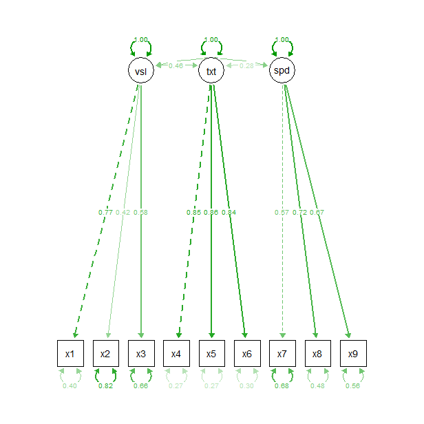
model <- "
visual  =~ x1 + x2 + x3
textual =~ x4 + x5 + x6
speed   =~ x7 + x8 + x9
"
fit <- cfa(model, data = HolzingerSwineford1939)
summary(fit, fit.measures = TRUE)
> summary(fit, fit.measures = TRUE)
lavaan (0.5-15) converged normally after  35 iterations

  Number of observations                           301

  Estimator                                         ML
  Minimum Function Test Statistic               85.306
  Degrees of freedom                                24
  P-value (Chi-square)                           0.000

Model test baseline model:

  Minimum Function Test Statistic              918.852
  Degrees of freedom                                36
  P-value                                        0.000

User model versus baseline model:

  Comparative Fit Index (CFI)                    0.931
  Tucker-Lewis Index (TLI)                       0.896

Loglikelihood and Information Criteria:

  Loglikelihood user model (H0)              -3737.745
  Loglikelihood unrestricted model (H1)      -3695.092

  Number of free parameters                         21
  Akaike (AIC)                                7517.490
  Bayesian (BIC)                              7595.339
  Sample-size adjusted Bayesian (BIC)         7528.739

Root Mean Square Error of Approximation:

  RMSEA                                          0.092
  90 Percent Confidence Interval          0.071  0.114
  P-value RMSEA <= 0.05                          0.001

Standardized Root Mean Square Residual:

  SRMR                                           0.065

Parameter estimates:

  Information                                 Expected
  Standard Errors                             Standard

                   Estimate  Std.err  Z-value  P(>|z|)
Latent variables:
  visual =~
    x1                1.000
    x2                0.554    0.100    5.554    0.000
    x3                0.729    0.109    6.685    0.000
  textual =~
    x4                1.000
    x5                1.113    0.065   17.014    0.000
    x6                0.926    0.055   16.703    0.000
  speed =~
    x7                1.000
    x8                1.180    0.165    7.152    0.000
    x9                1.082    0.151    7.155    0.000

Covariances:
  visual ~~
    textual           0.408    0.074    5.552    0.000
    speed             0.262    0.056    4.660    0.000
  textual ~~
    speed             0.173    0.049    3.518    0.000

Variances:
    x1                0.549    0.114
    x2                1.134    0.102
    x3                0.844    0.091
    x4                0.371    0.048
    x5                0.446    0.058
    x6                0.356    0.043
    x7                0.799    0.081
    x8                0.488    0.074
    x9                0.566    0.071
    visual            0.809    0.145
    textual           0.979    0.112
    speed             0.384    0.086

>
library(semPlot)
semPaths(fit,
         what="std",
         edge.label.cex = 0.6,
         sizeMan=5,
         sizeLat=5,
         curve=0.4
)
ى•„ëکى™€ ê°™ى´ ي‘œيک„ي• ىˆک ىˆىœ¼ë‚ک, ى—†ى–´ى§ˆ ي•¨ىˆکë¼ê³ ي•¨.
library(qgraph)
qgraph.lavaan(fit, layout="tree", titles=F,
              vsize.man=5,
              vsize.lat=5,
              filetype="",
              include=4,
              curve=-0.4,
              edge.label.cex=0.6)
[edit]
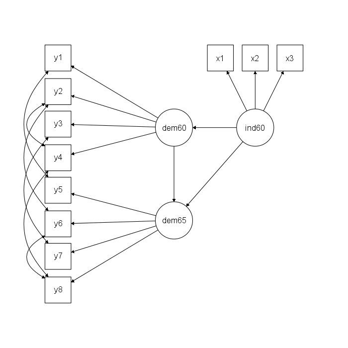
3 구ى،°ë°©ى •ى‹(SEM, structural equation modeling) #
PoliticalDemocracy ëچ°ى´ي„°ë¥¼ ى‚¬ىڑ©ي•œë‹¤. PoliticalDemocracyى—گ 대ي•œ ى„¤ëھ…ى€ ى—¬ê¸°ë¥¼ ى°¸ê³ ي•œë‹¤.
ى—¬ê¸°ë¥¼ ى°¸ê³ ي•œë‹¤.
library("lavaan")
data(PoliticalDemocracy)
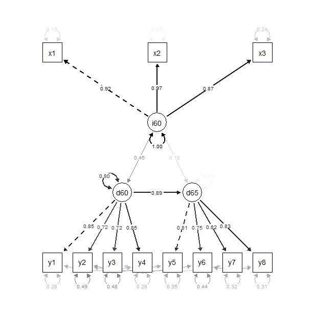
model <- "
# measurement model
ind60 =~ x1 + x2 + x3
dem60 =~ y1 + y2 + y3 + y4
dem65 =~ y5 + y6 + y7 + y8
# regressions
dem60 ~ ind60
dem65 ~ ind60 + dem60
# residual correlations
y1 ~~ y5
y2 ~~ y4 + y6
y3 ~~ y7
y4 ~~ y8
y6 ~~ y8
"
fit <- sem(model, data = PoliticalDemocracy)
summary(fit, standardized = TRUE)
> summary(fit, standardized = TRUE)
lavaan (0.5-15) converged normally after  68 iterations

  Number of observations                            75

  Estimator                                         ML
  Minimum Function Test Statistic               38.125
  Degrees of freedom                                35
  P-value (Chi-square)                           0.329

Parameter estimates:

  Information                                 Expected
  Standard Errors                             Standard

                   Estimate  Std.err  Z-value  P(>|z|)   Std.lv  Std.all
Latent variables:
  ind60 =~
    x1                1.000                               0.670    0.920
    x2                2.180    0.139   15.742    0.000    1.460    0.973
    x3                1.819    0.152   11.967    0.000    1.218    0.872
  dem60 =~
    y1                1.000                               2.223    0.850
    y2                1.257    0.182    6.889    0.000    2.794    0.717
    y3                1.058    0.151    6.987    0.000    2.351    0.722
    y4                1.265    0.145    8.722    0.000    2.812    0.846
  dem65 =~
    y5                1.000                               2.103    0.808
    y6                1.186    0.169    7.024    0.000    2.493    0.746
    y7                1.280    0.160    8.002    0.000    2.691    0.824
    y8                1.266    0.158    8.007    0.000    2.662    0.828

Regressions:
  dem60 ~
    ind60             1.483    0.399    3.715    0.000    0.447    0.447
  dem65 ~
    ind60             0.572    0.221    2.586    0.010    0.182    0.182
    dem60             0.837    0.098    8.514    0.000    0.885    0.885

Covariances:
  y1 ~~
    y5                0.624    0.358    1.741    0.082    0.624    0.296
  y2 ~~
    y4                1.313    0.702    1.871    0.061    1.313    0.273
    y6                2.153    0.734    2.934    0.003    2.153    0.356
  y3 ~~
    y7                0.795    0.608    1.308    0.191    0.795    0.191
  y4 ~~
    y8                0.348    0.442    0.787    0.431    0.348    0.109
  y6 ~~
    y8                1.356    0.568    2.386    0.017    1.356    0.338

Variances:
    x1                0.082    0.019                      0.082    0.154
    x2                0.120    0.070                      0.120    0.053
    x3                0.467    0.090                      0.467    0.239
    y1                1.891    0.444                      1.891    0.277
    y2                7.373    1.374                      7.373    0.486
    y3                5.067    0.952                      5.067    0.478
    y4                3.148    0.739                      3.148    0.285
    y5                2.351    0.480                      2.351    0.347
    y6                4.954    0.914                      4.954    0.443
    y7                3.431    0.713                      3.431    0.322
    y8                3.254    0.695                      3.254    0.315
    ind60             0.448    0.087                      1.000    1.000
    dem60             3.956    0.921                      0.800    0.800
    dem65             0.172    0.215                      0.039    0.039

>
library(semPlot)
semPaths(fit,
         what="std",
         edge.label.cex = 0.6,
         sizeMan=5,
         sizeLat=5,
         curve=0.4,
         edge.color="black"
)
[edit]
4.1 intercept #
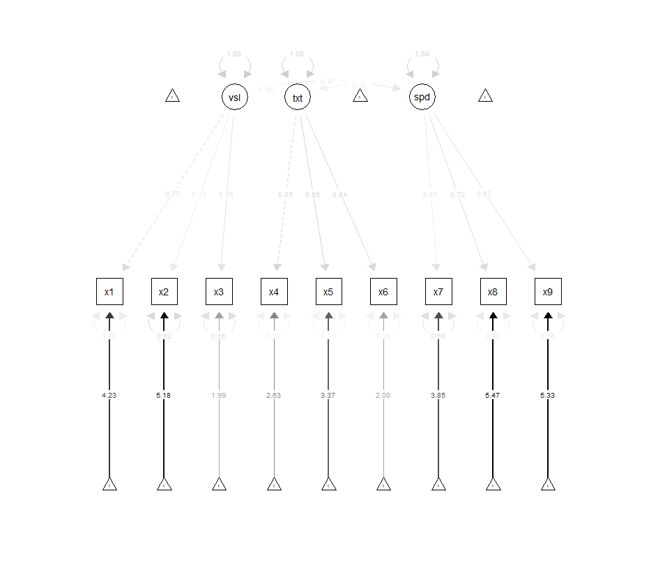
model <- "
# three-factor model
visual  =~ x1 + x2 + x3
textual =~ x4 + x5 + x6
speed   =~ x7 + x8 + x9

# intercepts
x1 ~ 1
x2 ~ 1
x3 ~ 1
x4 ~ 1
x5 ~ 1
x6 ~ 1
x7 ~ 1
x8 ~ 1
x9 ~ 1
"
fit <- cfa(model, data = HolzingerSwineford1939, meanstructure=T)
summary(fit, fit.measures = TRUE)

library(semPlot)
semPaths(fit,
         what="std",
         edge.label.cex = 0.6,
         sizeMan=5,
         sizeLat=5,
         curve=0.4,
         edge.color="black"
)
[edit]
4.2 group #
model <- "
# three-factor model
visual  =~ x1 + x2 + x3
textual =~ x4 + x5 + x6
speed   =~ x7 + x8 + x9
"
fit <- cfa(model, data = HolzingerSwineford1939, group="school")
summary(fit, fit.measures = TRUE)
[edit]
4.3 starting value #
model <- "
# three-factor model
visual  =~ x1 + 0.5*x2 + c(0.6, 0.8)*x3
textual =~ x4 + start(c(1.2, 0.6))*x5 + a*x6
speed   =~ x7 + x8 + x9
"
fit <- cfa(model, data = HolzingerSwineford1939, group="school")
summary(fit, fit.measures = TRUE)
starting valueê°€ 0.5*x2ê°™ى´ ىƒپىˆکë،œ ى£¼ى–´ ى§ˆ ىˆک ىˆë‹¤. ëکگي•œ c(0.6, 0.8)ى™€ ê°™ى´ ë²،ي„°ë،œ group별ë،œ starting value를 ë”°ë،œ ى¤„ ىˆک ىˆë‹¤.
[edit]
4.4 fitting function #
HS.model <- '  visual =~ x1 + x2 + x3
              textual =~ x4 + x5 + x6
              speed   =~ x7 + x8 + x9 '
fit <- cfa(HS.model,
           data = HolzingerSwineford1939,
           group = "school",
           group.equal = c("loadings"))
summary(fit)
group.equalى—گ loadings 대ى‹ 다ىŒê³¼ ê°™ى€ 것들ى´ ىک¬ ىˆک ىˆë‹¤. - intercepts: the intercepts of the observed variables
- means: the intercepts/means of the latent variables
- residuals: the residual variances of the observed variables
- residual.covariances: the residual covariances of the observed variables
- lv.variances: the (residual) variances of the latent variables
- lv.covariances: the (residual) covariances of the latent varibles
- regressions: all regression coefficients in the model
But what if you want to constrain a whole group of parameters (say all factor loadings and intercepts) across groups, except for one or two parameters that need to stay free in all groups. For this scenario, you can use the argument group.partial, containing the names of those parameters that need to remain free. For example:
fit <- cfa(HS.model,
           data = HolzingerSwineford1939,
           group = "school",
           group.equal = c("loadings", "intercepts"),
           group.partial = c("visual=~x2", "x7~1"))
[edit]
4.5 invariance #
library(semTools)
measurementInvariance(HS.model, data = HolzingerSwineford1939, group = "school")
[edit]
5 ىکˆى œ1 #
ى°¸ê³ : http://r-project.kr/content/r%EB%A1%9C-%ED%95%98%EB%8A%94-%EA%B5%AC%EC%A1%B0%EB%B0%A9%EC%A0%95%EC%8B%9D-lavaan2amos 문ى„œë¥¼ ë³´ê³ ي•¨.
library(lavaan)
> str(ch9.ex1)
'data.frame': 8 obs. of 5 variables:
$ attitude: int 2 3 3 4 4 4 4 5
$ loyalty : int 2 3 3 4 4 5 4 5
$ price : int 4 4 3 3 2 2 1 1
$ quality : int 2 3 2 3 3 4 3 5
$ design : int 2 3 4 2 5 3 2 4
> ch9.ex1
attitude loyalty price quality design
1 2 2 4 2 2
2 3 3 4 3 3
3 3 3 3 2 4
4 4 4 3 3 2
5 4 4 2 3 5
6 4 5 2 4 3
7 4 4 1 3 2
8 5 5 1 5 4
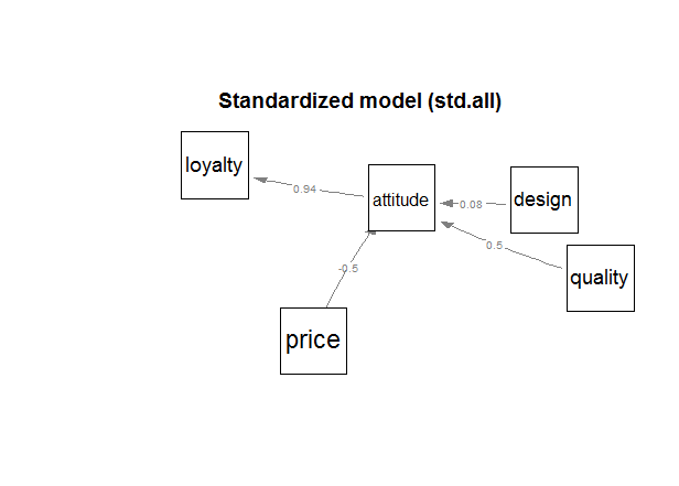
> path.model <- "
+ #regressions
+ attitude ~ price + quality + design
+ loyalty ~ attitude
+
+ #residual covariances
+ price ~~ quality
+ price ~~ design
+ quality ~~ design
+ "
> path.example <- lavaan(path.model, data=ch9.ex1, auto.var=T, auto.fix.first=T, fixed.x=F)
> summary(path.example)
lavaan (0.5-15) converged normally after 43 iterations
Number of observations 8
Estimator ML
Minimum Function Test Statistic 1.718
Degrees of freedom 3
P-value (Chi-square) 0.633
Parameter estimates:
Information Expected
Standard Errors Standard
Estimate Std.err Z-value P(>|z|)
Regressions:
attitude ~
price -0.382 0.133 -2.869 0.004
quality 0.459 0.159 2.883 0.004
design 0.063 0.109 0.579 0.562
loyalty ~
attitude 1.064 0.135 7.906 0.000
Covariances:
price ~~
quality -0.688 0.440 -1.563 0.118
design -0.313 0.431 -0.725 0.468
quality ~~
design 0.234 0.355 0.660 0.509
Variances:
attitude 0.097 0.048
loyalty 0.106 0.053
price 1.250 0.625
quality 0.859 0.430
design 1.109 0.555
> summary(path.example, fit.measures=T)
lavaan (0.5-15) converged normally after 43 iterations
Number of observations 8
Estimator ML
Minimum Function Test Statistic 1.718
Degrees of freedom 3
P-value (Chi-square) 0.633
Model test baseline model:
Minimum Function Test Statistic 40.609
Degrees of freedom 10
P-value 0.000
User model versus baseline model:
Comparative Fit Index (CFI) 1.000
Tucker-Lewis Index (TLI) 1.140
Loglikelihood and Information Criteria:
Loglikelihood user model (H0) -36.520
Loglikelihood unrestricted model (H1) -35.662
Number of free parameters 12
Akaike (AIC) 97.041
Bayesian (BIC) 97.994
Sample-size adjusted Bayesian (BIC) 62.535
Root Mean Square Error of Approximation:
RMSEA 0.000
90 Percent Confidence Interval 0.000 0.481
P-value RMSEA <= 0.05 0.641
Standardized Root Mean Square Residual:
SRMR 0.021
Parameter estimates:
Information Expected
Standard Errors Standard
Estimate Std.err Z-value P(>|z|)
Regressions:
attitude ~
price -0.382 0.133 -2.869 0.004
quality 0.459 0.159 2.883 0.004
design 0.063 0.109 0.579 0.562
loyalty ~
attitude 1.064 0.135 7.906 0.000
Covariances:
price ~~
quality -0.688 0.440 -1.563 0.118
design -0.313 0.431 -0.725 0.468
quality ~~
design 0.234 0.355 0.660 0.509
Variances:
attitude 0.097 0.048
loyalty 0.106 0.053
price 1.250 0.625
quality 0.859 0.430
design 1.109 0.555
> summary(path.example, standardized=T)
lavaan (0.5-15) converged normally after 43 iterations
Number of observations 8
Estimator ML
Minimum Function Test Statistic 1.718
Degrees of freedom 3
P-value (Chi-square) 0.633
Parameter estimates:
Information Expected
Standard Errors Standard
Estimate Std.err Z-value P(>|z|) Std.lv Std.all
Regressions:
attitude ~
price -0.382 0.133 -2.869 0.004 -0.382 -0.498
quality 0.459 0.159 2.883 0.004 0.459 0.497
design 0.063 0.109 0.579 0.562 0.063 0.078
loyalty ~
attitude 1.064 0.135 7.906 0.000 1.064 0.942
Covariances:
price ~~
quality -0.688 0.440 -1.563 0.118 -0.688 -0.663
design -0.313 0.431 -0.725 0.468 -0.313 -0.265
quality ~~
design 0.234 0.355 0.660 0.509 0.234 0.240
Variances:
attitude 0.097 0.048 0.097 0.132
loyalty 0.106 0.053 0.106 0.113
price 1.250 0.625 1.250 1.000
quality 0.859 0.430 0.859 1.000
design 1.109 0.555 1.109 1.000
> library(qgraph)
Warning message:
يŒ¨ي‚¤ى§€ â€کqgraph’ëٹ” R 버ى „ 3.0.3ى—گى„œ ى‘ى„±ëگکى—ˆىٹµë‹ˆë‹¤
> qgraph.lavaan(path.example, layout="spring",
+ vsize.man=8,
+ vsize.lat=8,
+ filetype="",
+ include=4,
+ curve=-0.4,
+ edge.label.cex=0.6)
- 브ëœë“œى—گ 대ي•œ يƒœëڈ„(attitude)ى—گ ىکپي–¥ى„ ى£¼ëٹ” ىڑ”ى¸ى€ 가격(price), ي’ˆى§ˆ(quality), ى™¸يک•(design)ى¸ëچ°,
- 가격ى€ ë‚®ى„ ىˆکë، ى¢‹ë‹¤. (-0.5)
- ي’ˆى§ˆëٹ” ى¢‹ى„ ىˆکë، ى¢‹ë‹¤. (0.5)
- ى™¸يک•ى€ 별ë،œ 관계가 ى—†ë‹¤. (0.08)
- 가격ى€ ë‚®ى„ ىˆکë، ى¢‹ë‹¤. (-0.5)
- ى¶©ى„±ëڈ„(royalty)ëٹ” 브ëœë“œى—گ 대ي•œ يƒœëڈ„ê°€ ىکپي–¥ى„ ى£¼ëٹ” ىڑ”ى¸ى´ë‹¤. (0.94)
[edit]
6 ىکˆى œ2 #
http://www.inside-r.org/packages/cran/qgraph/docs/qgraph.lavaan
## Not run:
## The industrialization and Political Democracy Example
# Example from lavaan::sem help file:
require("lavaan")
     ## Bollen (1989), page 332
     model <- '
       # latent variable definitions
          ind60 =~ x1 + x2 + x3
          dem60 =~ y1 + y2 + y3 + y4
          dem65 =~ y5 + equal("dem60=~y2")*y6
                      + equal("dem60=~y3")*y7
                      + equal("dem60=~y4")*y8

       # regressions
         dem60 ~ ind60
         dem65 ~ ind60 + dem60

       # residual correlations
         y1 ~~ y5
         y2 ~~ y4 + y6
         y3 ~~ y7
         y4 ~~ y8
         y6 ~~ y8
     '

     fit <- sem(model, data=PoliticalDemocracy)

# Plot standardized model (numerical):
qgraph.lavaan(fit,layout="tree",vsize.man=5,vsize.lat=10,
    filetype="",include=4,curve=-0.4,edge.label.cex=0.6)

# Plot standardized model (graphical):
qgraph.lavaan(fit,layout="tree",vsize.man=5,vsize.lat=10,
    filetype="",include=8,curve=-0.4,edge.label.cex=0.6)

# Create output document:
qgraph.lavaan(fit,layout="spring",vsize.man=5,vsize.lat=10,
    filename="lavaan")

## End(Not run)
[edit]
7 ى°¸ê³ ىگ료 #
- http://sachaepskamp.com/semPlot/examples --> semPlot Example
- 구ى،°ë°©ى •ى‹ى—گ 대ي•œ ى„¤ëھ…, يˆë“ ê·¸ë ˆى´ىٹ¤
- http://lavaan.ugent.be/tutorial/index.html
- https://personality-project.org/r/r.sem.html
- http://www.r-project.org/conferences/useR-2010/slides/Rosseel.pdf
- http://cran.r-project.org/doc/contrib/Fox-Companion/appendix-sems.pdf
 R구ى،°ë°©ى •ى‹.zip
- http://r-project.kr/content/r%EB%A1%9C-%ED%95%98%EB%8A%94-%EA%B5%AC%EC%A1%B0%EB%B0%A9%EC%A0%95%EC%8B%9D-lavaan2amos
- http://datawaffle.com/f_BigData/4332
- http://kimcw.khu.ac.kr/contents/bbs/bbs_content.html?bbs_cls_cd=007&cid=13031810035712&bbs_type=B
- http://www.ktcloudware.com/seminar/down/06.pdf
ï»؟