[edit]
2 мҳҲм ңлҚ°мқҙн„° #
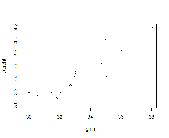
н—ҲлҰ¬л‘ҳл Ҳ(girth)мҷҖ лӘёл¬ҙкІҢ(weigth)
tmp <- textConnection(
"girth  weight
35.00  3.45
32.00	3.20
30.00	3.00
31.50	3.20
32.70	3.30
30.00	3.20
36.00	3.85
30.50	3.15
34.70	3.65
30.50	3.40
33.00	3.50
35.00	4.00
31.80	3.10
38.00	4.20
33.00	3.45")
x <- read.table(tmp, header=TRUE)
close.connection(tmp)
plot(x)
мӮ°м җлҸ„
![[http]](/moniwiki/imgs/http.png)
