[edit]
1 z нҶөкі„лҹү #
- 90% мӢ лў°кө¬к°„м—җм„ң z=1.645
- 95% мӢ лў°кө¬к°„м—җм„ң z=1.960
- 99% мӢ лў°кө¬к°„м—җм„ң z=1.2.576
[edit]
2 л№ лҘё мҳӨм°Ё кі„мӮ° #
AмӮ¬м•Ҳм—җ лҢҖн•ҙ мһ„мқҳлЎң м„ нғқлҗң көӯлҜјл“Ө 1000лӘ… мӨ‘м—җ 300лӘ…мқҙ м°¬м„ұн–ҲлӢӨ. мҳӨм°ЁлҠ”?
- 1/sqrt(1000) --> Вұ3.2%
[edit]
3 modified wald method лЎң мӢ лў°кө¬к°„ кө¬н•ҳкё° #
- z * sqrt(p * (1-p) / (n+z^2))
- мң„ мҳҲм ңм—җм„ңлҠ”.. 1.96 * sqrt(0.3 * (1-0.3) / (1000+1.96^2))
[edit]
4 1-sampleмқҳ 비мңЁ кІҖм • #
AкөҗмӢӨмқҳ н•ҷмғқмқҙ 100лӘ…мқҙ мһҲлӢӨ. мқҙмӨ‘ мҳӨлҘёмҶҗ мһЎмқҙлҠ” 86лӘ…мқҙлӢӨ. н•ңкөӯмқҖ 94%к°Җ мҳӨлҘёмҶҗ мһЎмқҙлӢӨ. н•ңкөӯкіј AкөҗмӢӨмқҳ н•ҷмғқл“Өмқҳ мҳӨлҘёмҶҗ мһЎмқҙ 비мңЁмқҖ к°ҷлӮҳ?
> prop.test(86,100,p=0.94)

	1-sample proportions test with continuity correction

data:  86 out of 100, null probability 0.94
X-squared = 9.9734, df = 1, p-value = 0.001588
alternative hypothesis: true p is not equal to 0.94
95 percent confidence interval:
 0.7728837 0.9185961
sample estimates:
   p
0.86
- мң мқҳмҲҳмӨҖ 0.05м—җм„ң лҢҖлҰҪк°Җм„Ө мұ„нғқ.
z.test <- function(x,n,p=NULL,conf.level=0.95,alternative="less") {
  ts.z <- NULL
  cint <- NULL
  p.val <- NULL
  phat <- x/n
  qhat <- 1 - phat
  # If you have p0 from the population or H0, use it.
  # Otherwise, use phat and qhat to find SE.phat:
  if(length(p) > 0) {
    q <- 1-p
    SE.phat <- sqrt((p*q)/n)
    ts.z <- (phat - p)/SE.phat
    p.val <- pnorm(ts.z)
    if(alternative=="two.sided") {
      p.val <- p.val * 2
    }
    if(alternative=="greater") {
      p.val <- 1 - p.val
    }
  } else {
    # If all you have is your sample, use phat to find
    # SE.phat, and don't run the hypothesis test:
    SE.phat <- sqrt((phat*qhat)/n)
  }
  cint <- phat + c(
    -1*((qnorm(((1 - conf.level)/2) + conf.level))*SE.phat),
    ((qnorm(((1 - conf.level)/2) + conf.level))*SE.phat) )
  return(list(estimate=phat,ts.z=ts.z,p.val=p.val,cint=cint))
}

z.test(86,100,p=0.94)
> z.test(86,100,p=0.94)
$estimate
[1] 0.86

$ts.z
[1] -3.368608

$p.val
[1] 0.0003777444

$cint
[1] 0.8134534 0.9065466
[edit]
5 nк°ңмқҳ 집лӢЁ 비мңЁм—җ лҢҖн•ң кІҖм • #
AлҸ„мӢңм—җм„ңлҠ” 300лӘ… мӨ‘ 100лӘ…мқҙ, BлҸ„мӢңм—җм„ңлҠ” 400лӘ… мӨ‘ 170лӘ…мқҙ Dнӣ„ліҙлҘј м§Җм§Җн•ңлӢӨкі мЎ°мӮ¬лҗҳм—ҲлӢӨ. AлҸ„мӢңмҷҖ BлҸ„мӢңмқҳ Dнӣ„л¶Җ м§Җм§Җ 비мңЁмқҙ к°ҷлӢӨкі н• мҲҳ мһҲлҠ”к°Җ?
분мһҗ <- c(100, 170) 분лӘЁ <- c(300, 400) prop.test(분мһҗ, 분лӘЁ)
> prop.test(분мһҗ, 분лӘЁ) 2-sample test for equality of proportions with continuity correction data: 분мһҗ out of 분лӘЁ X-squared = 5.6988, df = 1, p-value = 0.01698 alternative hypothesis: two.sided 95 percent confidence interval: -0.16664176 -0.01669158 sample estimates: prop 1 prop 2 0.3333333 0.4250000
кІ°кіјн•ҙм„қ
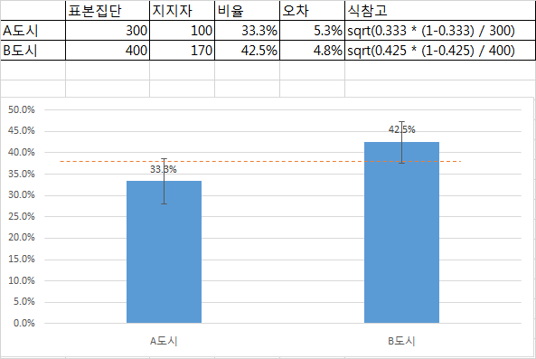
- л‘җ 집лӢЁм—җм„ң м–ҙл–Ө мӮ¬кұҙм—җ лҢҖн•ң 비мңЁмқҙ к°ҷлӢӨкі н• мҲҳ мһҲлҠ”м§Җм—җ лҢҖн•ң кІҖм •.
- к°Җм„Ө
- к·Җл¬ҙк°Җм„Ө: м°Ёмқҙк°Җ м—ҶлӢӨ.
- лҢҖлҰҪк°Җм„Ө: м°Ёмқҙк°Җ мһҲлӢӨ. --> мң мқҳмҲҳмӨҖ 0.05м—җм„ңлҠ” лҢҖлҰҪк°Җм„Ө м§Җм§Җ, мң мқҳмҲҳмӨҖ 0.01м—җм„ңлҠ” лҢҖлҰҪк°Җм„Ө кё°к°Ғ
- к·Җл¬ҙк°Җм„Ө: м°Ёмқҙк°Җ м—ҶлӢӨ.
- 95% мӢ лў°кө¬к°„: 0.4250000-0.16664176 ~ 0.4250000-0.01669158 = 0.2583582 ~ 0.4083084, кё°мӨҖмқҖ 100/300
[edit]
6 л°ңмғқмңЁ(Exact Poisson tests) #
м№ҙмҡҙнҠё лҚ°мқҙн„°м—җ лҢҖн•ҙ..
> poisson.test(분мһҗ, 분лӘЁ) Comparison of Poisson rates data: 분мһҗ time base: 분лӘЁ count1 = 100, expected count1 = 115.71, p-value = 0.05656 alternative hypothesis: true rate ratio is not equal to 1 95 percent confidence interval: 0.6064139 1.0099403 sample estimates: rate ratio 0.7843137
1н‘ңліё
> poisson.test(83, 100)

	Exact Poisson test

data:  83 time base: 100
number of events = 83, time base = 100, p-value = 0.09854
alternative hypothesis: true event rate is not equal to 1
95 percent confidence interval:
 0.6610904 1.0289099
sample estimates:
event rate
      0.83
- к·Җл¬ҙк°Җм„Ө: лӘЁм§‘лӢЁ л°ңмғқлҘ (О»)мқҙ к·Җл¬ҙ к°Җм„Өм—җм„ңмқҳ л°ңмғқлҘ кіј к°ҷлӢӨ.
- лҢҖлҰҪк°Җм„Ө: лӘЁм§‘лӢЁ л°ңмғқлҘ (О»)мқҙ к·Җл¬ҙ к°Җм„Өм—җм„ңмқҳ л°ңмғқлҘ кіј лӢӨлҘҙлӢӨ.
- мң мқҳмҲҳмӨҖ 0.05м—җм„ң к·Җл¬ҙк°Җм„Ө м§Җм§Җ
п»ҝ