Contents

1 개요

2 예제

3 다른 방법

4 참고자료

• 변수그룹(X={x1,x2, x3}, Y={y1,y2,y3}) 간의 선형관계 파악
  
• 어디서 주워들은 바로는 "주성분분석 + 회귀분석"
  

tmp <- textConnection( 
  "tv  디자인  기능성	매력도	선호도
  1	46	34	28	39
  2	60	31	50	46
  3	81	59	63	72
  4	94	84	92	92
  5	76	67	86	52
  6	31	53	41	39
  7	34	38	25	25
  8	78	75	64	76
  9	54	43	38	55
  10	86	53	60	70
  11	53	43	34	42
  12	78	31	52	67
  13	96	66	77	88
  14	71	90	86	65
  15	67	58	60	70
  16	32	68	74	45
  17	44	55	60	42
  18	59	46	42	67
  19	76	30	37	64
  20	84	51	54	79")
x <- read.table(tmp, header=TRUE) 
close.connection(tmp)
#head(x)

library("sqldf")
d1 <- sqldf("select 디자인, 기능성 from x")
d2 <- sqldf("select 매력도, 선호도 from x")
rs1 <- cancor(d1, d2)
rs1$cor

> X <- with(x, -0.007865095 * (디자인-65.00) + -0.006951716 * (기능성-53.75))
> Y <- with(x, -0.007865095 * (매력도-56.15) + -0.006951716 * (선호도-59.75))
> cor.test(X,Y)

	Pearson's product-moment correlation

data:  X and Y
t = 13.0087, df = 18, p-value = 1.362e-10
alternative hypothesis: true correlation is not equal to 0
95 percent confidence interval:
 0.8772728 0.9806609
sample estimates:
      cor 
0.9507151 

> plot(X,Y)

#install.packages("CCA")
library("CCA")
rs2 <- cc(d1, d2)
plot(rs2$scores$xscores[,1], rs2$scores$yscores[,1])

#install.packages("yacca")
library("yacca")
rs3 <- cca(d1, d2)
rs3

> rs3

Canonical Correlation Analysis

Canonical Correlations:
     CV 1      CV 2 
0.9558493 0.6976745 

X Coefficients:
              CV 1        CV 2
디자인 -0.03428316  0.03920114
기능성 -0.03030183 -0.05234068

Y Coefficients:
              CV 1        CV 2
매력도 -0.02577813 -0.05651435
선호도 -0.03411328  0.05890991

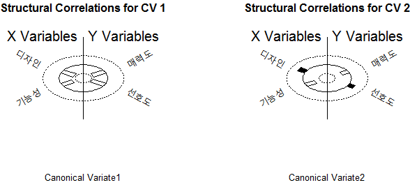
Structural Correlations (Loadings) - X Vars:
             CV 1       CV 2
디자인 -0.8654311  0.5010280
기능성 -0.7527465 -0.6583105

Structural Correlations (Loadings) - Y Vars:
             CV 1       CV 2
매력도 -0.8653783 -0.5011192
선호도 -0.9098212  0.4150005

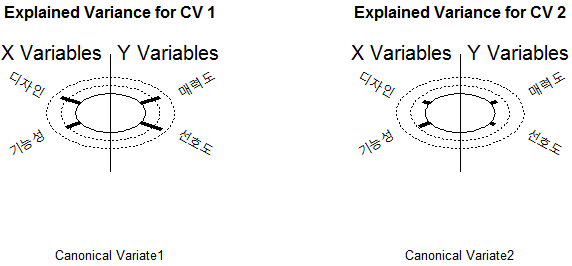
Aggregate Redundancy Coefficients (Total Variance Explained):
	X | Y: 0.7675629 
	Y | X: 0.823285

> plot(rs3)

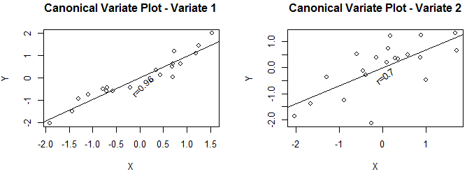
• 제1정준상관변수(CV1) - 변수그룹X와 변수그룹Y와의 최대 상관 계수는 0.96
  
• 제2정준상관변수(CV2) - 변수그룹X와 변수그룹Y와의 최대 상관 계수 다음으로 높은 상관계수는 0.7
  

Canonical Correlations:
     CV 1      CV 2 
0.9558493 0.6976745 

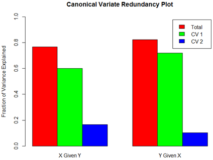
Aggregate Redundancy Coefficients (Total Variance Explained):
	X | Y: 0.7675629 
	Y | X: 0.823285

Structural Correlations (Loadings) - X Vars:
             CV 1       CV 2
디자인 -0.8654311  0.5010280
기능성 -0.7527465 -0.6583105

Structural Correlations (Loadings) - Y Vars:
             CV 1       CV 2
매력도 -0.8653783 -0.5011192
선호도 -0.9098212  0.4150005

• 정준적재(canonical loadings) - 검증하는 방법
  
• X그룹의 변수인 디자인, 기능성과 CV1, CV2의 상관계수
  
• Y그룹의 변수인 매력도, 선호도와 CV1, CV2의 상관계수
  
• 참고: 정준교차적재(canonical cross-loadings, 한 변수와 해당 변수그룹이 아닌 비교그룹의 정준상관변수와의 상관관계)라는 것도 있다.
  
  

X Coefficients:
              CV 1        CV 2
디자인 -0.03428316  0.03920114
기능성 -0.03030183 -0.05234068

Y Coefficients:
              CV 1        CV 2
매력도 -0.02577813 -0.05651435
선호도 -0.03411328  0.05890991

• CV1
  
  • X = -0.03428316 * 디자인 + -0.03030183 + 기능성
    
  • Y = -0.02577813 * 매력도 + -0.03411328 * 선호도
    
• CV2
  
  • X = 0.03920114 * 디자인 + -0.05234068 + 기능성
    
  • Y = -0.05651435 * 매력도 + 0.05890991 * 선호도
    
    

> X <- with(x, -0.03428316 * 디자인 + -0.03030183 * 기능성)
> Y <- with(x, -0.02577813 * 매력도 + -0.03411328 * 선호도)
> cor.test(X,Y)

	Pearson's product-moment correlation

data:  X and Y
t = 13.8003, df = 18, p-value = 5.156e-11
alternative hypothesis: true correlation is not equal to 0
95 percent confidence interval:
 0.8896248 0.9827032
sample estimates:
      cor 
0.9558493 

> F.test.cca(rs3)

	F Test for Canonical Correlations (Rao's F Approximation)

         Corr        F   Num df Den df    Pr(>F)    
CV 1  0.95585 30.00045  4.00000     32 2.029e-10 ***
CV 2  0.69767 16.12224  1.00000     17 0.0008971 ***
---
Signif. codes:  0 ‘***’ 0.001 ‘**’ 0.01 ‘*’ 0.05 ‘.’ 0.1 ‘ ’ 1 

• 제1정준상관변수, 제2정준상관변수 모두 쓸모있다.
  
  
  
  

• http://blog.naver.com/chcher?Redirect=Log&logNo=70138773767