[edit]
1 к°ңмҡ” #
Rмқ„ мқҙмҡ©н•ҙм„ң лҚ°мқҙн„° 집합мқҙ м–ҙл–Ө нҷ•лҘ 분нҸ¬мҷҖ к°Җк№Ңмҡҙм§Җ м•Ңм•„ліҙлҸ„лЎқ н•ҳмһҗ. нҷ•лҘ 분нҸ¬мқҳ м Ғн•©м„ұмқ„ м•Ңм•„ліҙл Өл©ҙ "fitdistrplus" PackageлҘј мқҙмҡ©н•ҳл©ҙ лҗңлӢӨ.
--SciPyмҷҖ NumPy, н•ңл№ӣлҜёл””м–ҙ, м—ҳлҰ¬ лёҢл Ҳм„ӨнҠё м§ҖмқҢ/мқҙм„ұмЈј мҳҜк№Җ
[edit]
2 fitdistrplus Package Install #
install.packages("fitdistrplus",dependencies=T)
library(fitdistrplus)
[edit]
3 мӮ¬мҡ©л°©лІ• #
лӢӨмқҢкіј к°ҷмқҖ нҷ•лҘ 분нҸ¬лҘј м•Ңм•„лӮј мҲҳ мһҲлӢӨ.
"norm", "lnorm", "exp", "pois", "cauchy", "gamma", "logis", "nbinom", "geom", "beta", "weibull"
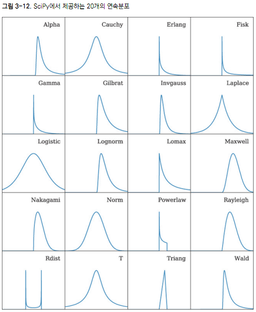
к·ёлҰјмңјлЎң ліҙкё°
"norm", "lnorm", "exp", "pois", "cauchy", "gamma", "logis", "nbinom", "geom", "beta", "weibull"
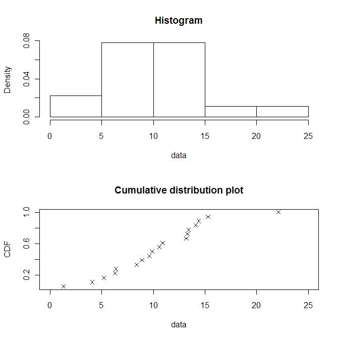
x1 <- c(6.4, 13.3, 4.1, 1.3, 14.1, 10.6, 9.9, 9.6, 15.3,
22.1,13.4, 13.2, 8.4, 6.3, 8.9, 5.2, 10.9, 14.4)
plotdist(x1)
descdist(x1)
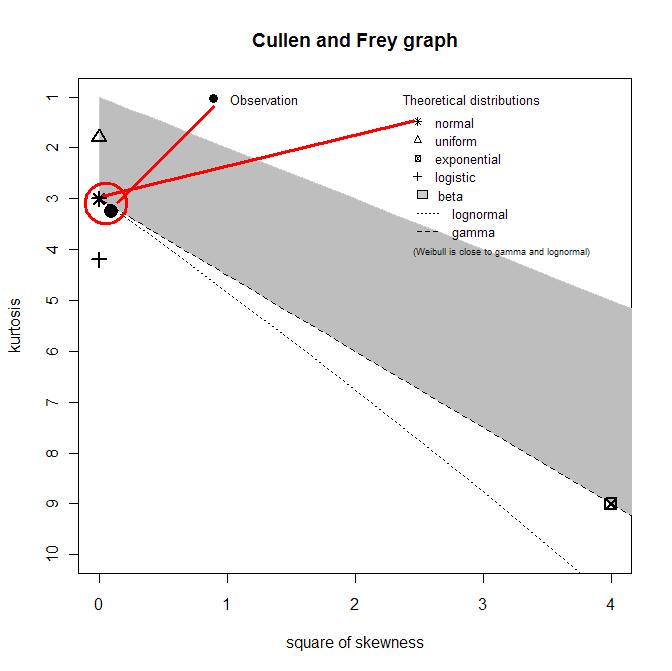
кҙҖмёЎм№ҳк°Җ м •к·ң분нҸ¬(normal)м—җ к°ҖмһҘ к°Җк№Ңмҡҙ кІғмқ„ ліј мҲҳ мһҲлӢӨ.
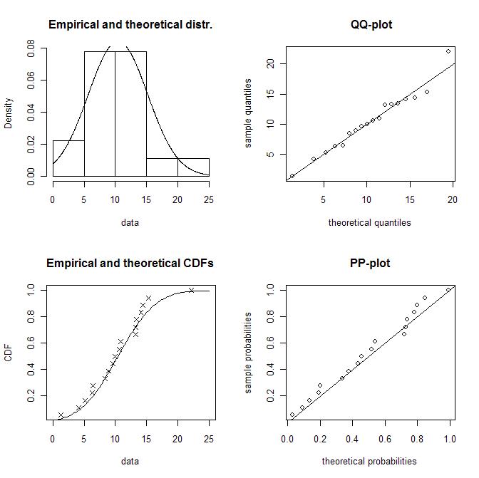
# "norm"лҢҖмӢ м—җ лӢӨмқҢкіј к°ҷмқҖ кІғл“Өмқ„ л„Јмқ„ мҲҳ мһҲлӢӨ. # "lnorm", "exp", "pois", "cauchy", "gamma", "logis", "nbinom", "geom", "beta", "weibull" f1 <- fitdist(x1, "norm") summary(f1) plot(f1) summary(gofstat(f1)) gofstat(f1)$chisqpvalue
summary(f1l)мқҳ кІ°кіјлҠ” лӢӨмқҢкіј к°ҷлӢӨ.
> summary(f1)
Fitting of the distribution ' norm ' by maximum likelihood
Parameters :
      estimate Std. Error
mean 10.411111   1.118886
sd    4.747033   0.791172
Loglikelihood:  -53.57625   AIC:  111.1525   BIC:  112.9332
Correlation matrix:
     mean sd
mean    1  0
sd      0  1
gofstat(f1)$chisqpvalueмқҳ кІ°кіјлҠ” лӢӨмқҢкіј к°ҷлӢӨ.
> gofstat(f1)
Kolmogorov-Smirnov statistic:  0.1104554
Cramer-von Mises statistic:  0.02848332
Anderson-Darling statistic:  0.225598
[1] 0.1847961
лӢӨмқҖ кІғмқҖ мһҳ лӘЁлҘҙкІ кі .. м№ҙмқҙм ңкіұ кІҖм •мқҳ p-valueлҠ” лӢӨмқҢкіј к°ҷмқҙ н•ҙм„қн• мҲҳ мһҲлӢӨ.
- Chi-squared p-value: 0.185
- к°Җм„Ө
- к·Җл¬ҙк°Җм„Ө: м°Ёмқҙк°Җ м—ҶлӢӨ. -> м •к·ң분нҸ¬лӢӨ.
- лҢҖлҰҪк°Җм„Ө: м°Ёмқҙк°Җ мһҲлӢӨ. -> м •к·ң분нҸ¬к°Җ м•„лӢҲлӢӨ.
- к·Җл¬ҙк°Җм„Ө: м°Ёмқҙк°Җ м—ҶлӢӨ. -> м •к·ң분нҸ¬лӢӨ.
- p-valueлҠ” лҢҖлҰҪк°Җм„Өмқҙ 1мў… мҳӨлҘҳк°Җ лӮҳнғҖлӮ нҷ•лҘ мқҙлӢӨ. p-value=0.185лЎң мң мқҳнҷ•лҘ 0.05ліҙлӢӨ нҒ¬лҜҖлЎң лҢҖлҰҪк°Җм„Өмқҙ нӢҖл ёлӢӨкі ліј мҲҳ мһҲлӢӨ. к·ёлҹ¬лҜҖлЎң к·Җл¬ҙк°Җм„Ө мұ„нғқ. мҰү, м •к·ң분нҸ¬лқјкі ліј мҲҳ мһҲлӢӨ.
н•ҳлӮҳмқҳ мҳҲм ңл§Ң лҚ” н•ҙліҙмһҗ. нҸ¬м•„мҶЎл¶„нҸ¬мқҳ м Ғн•©м„ұ 분м„қмқ„ н•ҙліҙмһҗ.
x2<-c(rep(4,1),rep(2,3),rep(1,7),rep(0,12))
gofstat(fitdist(x2,"pois"))$chisqpvalue
кІ°кіјлҠ” лӢӨмқҢкіј к°ҷлӢӨ.
Chi-squared statistic:  0.2507318
[1] 0.6165603
лӢӨлҘё кІғмқҖ мһҳ лӘЁлҘҙкІ кі , p-valueк°Җ 0.617лЎң лҢҖлҰҪк°Җм„Өмқҙ л»‘лӮ нҷ•лҘ мқҙ мЎ°лӮё лҶ’лӢӨ. к·ёлҹ¬лҜҖлЎң к·Җл¬ҙк°Җм„Өмқ„ м§Җм§Җн•ңлӢӨ. мҰү, нҸ¬м•„мҶЎ 분нҸ¬лӢӨ.
[edit]
4 м–ҙл–Ө 분нҸ¬м—җ к°Җк№Ңмҡҙк°Җ? #
options(show.error.messages = FALSE)
dist_name <- c()
p_value <- c()
dist <- c("norm", "lnorm", "pois", "exp", "gamma", "nbinom", "geom", "beta", "unif", "logis")
for(i in dist)
{
print(i)
f1 <- try(with(trees, fitdist(Height, i, method="mme")))
if(class(f1) == "try-error") next;
pval <- gofstat(f1)$chisqpvalue
if (pval >= 0.05)
{
print(paste("분нҸ¬лӘ…:", i, ", p-value =", as.character(pval)))
dist_name <- c(dist_name, i)
p_value <- c(p_value, pval)
}
}
print("chisq.test...")
print(data.frame(dist_name, p_value))
#with(trees, hist(Height))
with(trees, descdist(Height))
кІ°кіј
> print(data.frame(dist_name, p_value))
  dist_name p_value
1      norm   0.595
2     lnorm   0.537
3      pois   0.238
4     gamma   0.558
[edit]
5 м •к·ң분нҸ¬мқём§Җ м•„лӢҢм§Җ кІҖм • #
- к·Җл¬ҙк°Җм„Ө: м •к·ң분нҸ¬мҷҖ м°Ёмқҙк°Җ м—ҶлӢӨ.
- лҢҖлҰҪк°Җм„Ө: м •к·ң분нҸ¬мҷҖ м°Ёмқҙк°Җ мһҲлӢӨ.
> source("rftn.f")
> rad.d <-read.table("rad.d", header=T)
> shapiro.test(rad.d$open)

        Shapiro-Wilk normality test

data:  rad.d$open
W = 0.8292, p-value = 1.977e-05
p-value < 0.05 мқҙлҜҖлЎң м •к·ң분нҸ¬лҘј л”°лҘҙм§Җ м•ҠлҠ”лӢӨ.
ліҖмҲҳк°Җ мЎ°лӮё л§Һмқ„ кІҪмҡ°
install.packages("fBasics")
library("fBasics")
tmp <- rnorm(10000)
ksnormTest(tmp)
shapiroTest(tmp)
jarqueberaTest(tmp) #мқҙкІҢ мўӢкө¬лӮҳ~~!!!!
dagoTest(tmp)
- http://rss.acs.unt.edu/Rdoc/library/fBasics/html/NormalityTests.html
- ksnormTest - Kolmogorov-Smirnov normality test,
- shapiroTest - Shapiro-Wilk's test for normality,
- jarqueberaTest - JarqueвҖ“Bera test for normality,
- dagoTest - D'Agostino normality test.
![[http]](/moniwiki/imgs/http.png) anderson-darling test н•ҙлҸ„ лҗңлӢӨ. л№Ңм–ҙлЁ№мқ„ shapiro.testмқҳ 5,000кұҙ м ңн•ңмқ„ л„ҳкёё мҲҳ мһҲлӢӨ.
anderson-darling test н•ҙлҸ„ лҗңлӢӨ. л№Ңм–ҙлЁ№мқ„ shapiro.testмқҳ 5,000кұҙ м ңн•ңмқ„ л„ҳкёё мҲҳ мһҲлӢӨ.library(nortest) ad.test(rnorm(10000, mean = 5, sd = 3)) ad.test(runif(10000, min = 2, max = 4))
[edit]
6 к°ҷмқҖ 분нҸ¬м—җм„ң мҳЁ мғҳн”Ңмқёк°Җ? #
kolmogorov-smirnov testлҘј мқҙмҡ©н•ңлӢӨ.
x <- rnorm(100, mean = 0, sd = 1)
y <- rnorm(100, mean = 1, sd = 1)
ks.test(x,y)
> ks.test(x,y)

	Two-sample Kolmogorov-Smirnov test

data:  x and y
D = 0.38, p-value = 1.071e-06
alternative hypothesis: two-sided
- p-value = 1.071e-06 мқҙлҜҖлЎң к·Җл¬ҙк°Җм„Ө кё°к°Ғ. мҰү, л‘җ мғҳн”ҢмқҖ лӢӨлҘё лӘЁм§‘лӢЁ 분нҸ¬лӢӨ.
- 비лӘЁмҲҳ кІҖм •мңјлЎң лӘЁм§‘лӢЁм—җ лҢҖн•ң м–ҙл–Ө к°Җм •лҸ„ н•„мҡ”м—ҶлӢӨ.
[edit]
7 мқҙкұ° н•ҳлӮҳл©ҙ 충분 #
#install.packages("propagate")
library(propagate)
y <- c(0.0941,0.2372,0.2923,0.1750,0.0863,0.0419,0.0207,0.0128,0.0142,0.0071,0.0041,0.0031,0.0032,0.0057,0.0022,0.0001)
fit.result <- fitDistr(y)
fit.result
#лҸ„мӣҖл§җмқ„ м°ҫм•„ліҙл©ҙ н•ЁмҲҳмқҳ лӮҙмҡ©мқҙ л¬ҙм—Үмқём§Җ м•Ң мҲҳ мһҲлӢӨ.
print(propagate:::dJSB)
кІ°кіј
> fit.result <- fitDistr(y)
Fitting Normal distribution...Done.
Fitting Skewed-normal distribution...Done.
Fitting Generalized normal distribution...........10.........20.......Done.
Fitting Log-normal distribution...Done.
Fitting Scaled/shifted t- distribution...Done.
Fitting Logistic distribution...Done.
Fitting Uniform distribution...Done.
Fitting Triangular distribution...Done.
Fitting Trapezoidal distribution...Done.
Fitting Curvilinear Trapezoidal distribution...Done.
Fitting Generalized Trapezoidal distribution...Done.
Fitting Gamma distribution...Done.
Fitting Cauchy distribution...Done.
Fitting Laplace distribution...Done.
Fitting Gumbel distribution...Done.
Fitting Johnson SU distribution...........10.........20.........30.........40.........50
.........60.........70.........80.Done.
Fitting Johnson SB distribution...........10.........20.........30.........40.........50
.........60.........70.........80.Done.
Fitting 3P Weibull distribution...........10.........20.......Done.
Fitting 4P Beta distribution...Done.
Fitting Arcsine distribution...Done.
Fitting von Mises distribution...Done.
> fit.result
$aic
              Distribution      AIC
17              Johnson SB 613.7082
18              3P Weibull 624.7589
3       Generalized normal 624.7920
16              Johnson SU 626.7920
4               Log-normal 627.1804
12                   Gamma 634.9023
14                 Laplace 639.8102
13                  Cauchy 640.2875
5        Scaled/shifted t- 642.1013
15                  Gumbel 642.8420
2            Skewed-normal 646.8412
6                 Logistic 647.8476
1                   Normal 652.1788
9              Trapezoidal 654.7066
20                 Arcsine 670.4624
19                 4P Beta 705.6771
11 Generalized Trapezoidal 836.8772
21               von Mises 882.3921
7                  Uniform 897.6248
8               Triangular 905.4962
10 Curvilinear Trapezoidal 911.1446

$fit
$fit$Normal
Nonlinear regression via the Levenberg-Marquardt algorithm
parameter estimates: 0.000717984960447366, 0.00725890392042258
residual sum-of-squares: 197174
reason terminated: Relative error in the sum of squares is at most `ftol'.

$fit$`Skewed-normal`
Nonlinear regression via the Levenberg-Marquardt algorithm
parameter estimates: -0.00583038510142194, 0.0106443425236555, 8.50327745471171
residual sum-of-squares: 174116
reason terminated: Relative error in the sum of squares is at most `ftol'.

$fit$`Generalized normal`
Nonlinear regression via the Levenberg-Marquardt algorithm
parameter estimates: 0.0818148807363509, 0.0385147298611958, -2.26477841096039
residual sum-of-squares: 119822
reason terminated: Relative error in the sum of squares is at most `ftol'.

$fit$`Log-normal`
Nonlinear regression via the Levenberg-Marquardt algorithm
parameter estimates: -4.42473398922409, 2.05820723941306
residual sum-of-squares: 129074
reason terminated: Relative error in the sum of squares is at most `ftol'.

$fit$`Scaled/shifted t-`
Nonlinear regression via the Levenberg-Marquardt algorithm
parameter estimates: 0.002960556811455, 0.00543082394110837, 0.847275538361585
residual sum-of-squares: 160675
reason terminated: Relative error in the sum of squares is at most `ftol'.

$fit$Logistic
Nonlinear regression via the Levenberg-Marquardt algorithm
parameter estimates: 0.00106198716159507, 0.00448320432790849
residual sum-of-squares: 183218
reason terminated: Relative error in the sum of squares is at most `ftol'.

$fit$Uniform
Nonlinear regression via the Levenberg-Marquardt algorithm
parameter estimates: 0.00249994429141502, 0.289899967178183
residual sum-of-squares: 12634542
reason terminated: Relative error in the sum of squares is at most `ftol'.

$fit$Triangular
Nonlinear regression via the Levenberg-Marquardt algorithm
parameter estimates: -0.58442884603643, 0.276474920439136, 0.00750016053696837
residual sum-of-squares: 13956564
reason terminated: Relative error between `par' and the solution is at most `ptol'.

$fit$Trapezoidal
Nonlinear regression via the Levenberg-Marquardt algorithm
parameter estimates: -0.267697695351802, 0.162169769399358, -0.118546092194162, 0.0169541854752057
residual sum-of-squares: 192315
reason terminated: Relative error in the sum of squares is at most `ftol'.

$fit$`Curvilinear Trapezoidal`
Nonlinear regression via the Levenberg-Marquardt algorithm
parameter estimates: -3.51380272100041, 0.781019642275179, 0.778518731596065
residual sum-of-squares: 15358740
reason terminated: Relative error in the sum of squares is at most `ftol'.

$fit$`Generalized Trapezoidal`
Nonlinear regression via the Levenberg-Marquardt algorithm
parameter estimates: -0.316014522465303, -0.0122579620659835, 0.00250001098860818, -0.0569154565231172, 16.9883350504257, -13.687268319418, 1.38700131982915
residual sum-of-squares: 3808834
reason terminated: Relative error between `par' and the solution is at most `ptol'.

$fit$Gamma
Nonlinear regression via the Levenberg-Marquardt algorithm
parameter estimates: 0.365709818937871, 25.9401735353146
residual sum-of-squares: 147123
reason terminated: Relative error in the sum of squares is at most `ftol'.

$fit$Cauchy
Nonlinear regression via the Levenberg-Marquardt algorithm
parameter estimates: 0.0027034462361882, 0.00566077284092268
residual sum-of-squares: 161183
reason terminated: Relative error in the sum of squares is at most `ftol'.

$fit$Laplace
Nonlinear regression via the Levenberg-Marquardt algorithm
parameter estimates: 0.00208489337704117, 0.0115719008947262
residual sum-of-squares: 159884
reason terminated: Relative error in the sum of squares is at most `ftol'.

$fit$Gumbel
Nonlinear regression via the Levenberg-Marquardt algorithm
parameter estimates: -0.000564496234569831, 0.00585195632924723
residual sum-of-squares: 168315
reason terminated: Relative error in the sum of squares is at most `ftol'.

$fit$`Johnson SU`
Nonlinear regression via the Levenberg-Marquardt algorithm
parameter estimates: 0.00238945145777224, 2.41428652017113e-08, -6.58408257452447, 0.441518979946343
residual sum-of-squares: 119822
reason terminated: Relative error in the sum of squares is at most `ftol'.

$fit$`Johnson SB`
Nonlinear regression via the Levenberg-Marquardt algorithm
parameter estimates: 0.00249961631424682, 0.290585603944236, 0.633747903543896, 0.35472053982219
residual sum-of-squares: 95990
reason terminated: Relative error in the sum of squares is at most `ftol'.

$fit$`3P Weibull`
Nonlinear regression via the Levenberg-Marquardt algorithm
parameter estimates: 0.00206926024634554, 0.60287651598625, 0.0650136696113521
residual sum-of-squares: 119755
reason terminated: Relative error in the sum of squares is at most `ftol'.

$fit$`4P Beta`
Nonlinear regression via the Levenberg-Marquardt algorithm
parameter estimates: 243.96530522719, 244.003863012748, -0.219805373171359, 0.221019706262809
residual sum-of-squares: 456251
reason terminated: Relative error between `par' and the solution is at most `ptol'.

$fit$Arcsine
Nonlinear regression via the Levenberg-Marquardt algorithm
parameter estimates: 0.00241801362975452, 0.295326975917706
residual sum-of-squares: 268803
reason terminated: Relative error in the sum of squares is at most `ftol'.

$fit$`von Mises`
Nonlinear regression via the Levenberg-Marquardt algorithm
parameter estimates: 0.00235128799831663, 314.160915522474
residual sum-of-squares: 9759620
reason terminated: Number of iterations has reached `maxiter' == 1024.


$bestfit
Nonlinear regression via the Levenberg-Marquardt algorithm
parameter estimates: 0.00249961631424682, 0.290585603944236, 0.633747903543896, 0.35472053982219
residual sum-of-squares: 95990
reason terminated: Relative error in the sum of squares is at most `ftol'.

$fitted
 [1] 62.219673 20.891649 12.605071  9.187138  7.285103  6.065145  5.213740  4.585130  4.101920  3.719054  3.408463
[12]  3.151718  2.936210  2.753014  2.595632  2.459222  2.340100  2.235416  2.142929  2.060858  1.987768  1.922492
[23]  1.864074  1.811724  1.764788  1.722718  1.685056  1.651422  1.621494  1.595006  1.571740  1.551516  1.534193
[34]  1.519663  1.507852  1.498715  1.492237  1.488439  1.487372  1.489126  1.493832  1.501671  1.512883  1.527777
[45]  1.546754  1.570328  1.599166  1.634138  1.676391  1.727475  1.789524  1.865572  1.960094  2.080031  2.236881
[56]  2.451540  2.767639  3.300214  4.355798

$residuals
 [1]  0.2803273  4.1083505 12.3949289 -9.1871379  5.2148973 -6.0651453 -5.2137405 -4.5851299  8.3980803 -3.7190542
[11] -3.4084626 -3.1517175 -2.9362096 -2.7530136 -2.5956321 -2.4592222 -2.3401002 10.2645843 10.3570709 -2.0608580
[21] -1.9877677 -1.9224916 -1.8640737 -1.8117243 -1.7647878 -1.7227176 -1.6850565 -1.6514218 -1.6214937 -1.5950062
[31] -1.5717396 -1.5515155 -1.5341925 -1.5196632 10.9921481 -1.4987145 -1.4922374 -1.4884391 -1.4873721 -1.4891258
[41] -1.4938321 -1.5016714 -1.5128828 -1.5277768 -1.5467535 -1.5703281 -1.5991664 10.8658625 -1.6763910 -1.7274750
[51] -1.7895244 -1.8655720 -1.9600941 -2.0800311 -2.2368812 -2.4515397 -2.7676387 -3.3002136  8.1442017
м°ёкі : https://github.com/cran/propagate/blob/48a08079e6fdae6264809870867424ad698c49fc/R/distr-densities.R
############### distribution fitting ###################
## skew-normal distribution, taken from package 'VGAM'
dsn <- function (x, location = 0, scale = 1, shape = 0, log = FALSE)
{
  zedd <- (x - location)/scale
  loglik <- log(2) + dnorm(zedd, log = TRUE) + pnorm(shape * zedd, log.p = TRUE) - log(scale)
  if (log) loglik else exp(loglik)
}

## generalized normal distribution,
## taken from PDF in Mathematica's "Ultimate Univariate Probability Distribution Explorer"
dgnorm <- function(x, alpha = 1, xi = 1, kappa = -0.1)
{
  1/(exp(log(1 - (kappa * (x - xi))/alpha)^2/(2 * kappa^2)) * (sqrt(2 * pi) * (alpha - x * kappa + kappa * xi)))
}

## scaled and shifted t-distribution,
dst <- function (x, mean = 0, sd = 1, df = 2)
{
  dt((x - mean)/sd, df = df)/sd
}

## Gumbel distribution,
## taken from PDF in Mathematica's "Ultimate Univariate Probability Distribution Explorer"
dgumbel <- function(x, location = 0, scale = 1) {
  z <- (x - location)/scale
  (1/scale) * exp(-z - exp(-z))
}

## Johnson SU distribution,
## taken from PDF in Mathematica's "Ultimate Univariate Probability Distribution Explorer"
dJSU <- function (x, xi = 0, lambda = 1, gamma = 1, delta = 1)
{
  z <- (x - xi)/lambda
  delta/(lambda * sqrt(2 * pi) * sqrt(z^2 + 1)) * exp(-0.5 * (gamma + delta * log(z + sqrt(z^2 + 1)))^2)
}

## Johnson SB distribution,
## taken from PDF in Mathematica's "Ultimate Univariate Probability Distribution Explorer"
dJSB <- function (x, xi = 0, lambda = 1, gamma = 1, delta = 1)
{
  z <- (x - xi)/lambda
  delta/(lambda * sqrt(2 * pi) * z * (1 - z)) * exp(-0.5 * (gamma + delta * log(z/(1 - z)))^2)
}

## three-parameter weibull distribution with location gamma,
## taken from PDF in Mathematica's "Ultimate Univariate Probability Distribution Explorer"
dweibull2 <- function(x, location = 0, shape = 1, scale = 1) {
  (shape/scale) * ((x - location)/scale)^(shape - 1) * exp(-((x - location)/scale)^shape)
}

## four-parameter beta distribution with boundary parameters,
## taken from PDF in Mathematica's "Ultimate Univariate Probability Distribution Explorer"
dbeta2 <- function(x, alpha1 = 1, alpha2 = 1, a = 0, b = 0) {
  (1/beta(alpha1, alpha2)) * ((x - a)^(alpha1 - 1) * (b - x)^(alpha2 - 1))/(b - a)^(alpha1 + alpha2 - 1)
}

## triangular distribution,
## taken from PDF in Mathematica's "Ultimate Univariate Probability Distribution Explorer"
dtriang <- function(x, a = 0, b = 1, c = 2) {
  y <- numeric(length(x))
  y[x < a] <- 0
  y[a <= x & x <= b] <- 2 * (x[a <= x & x <= b] - a)/((c - a) * (b - a))
  y[b < x & x <= c] <- 2 * (c - x[b < x & x <= c])/((c - a) * (c - b))
  y[c < x] <- 0
  return(y)
}

## trapezoidal distribution,
## taken from PDF in Mathematica's "Ultimate Univariate Probability Distribution Explorer"
dtrap <- function(x, a = 0, b = 1, c = 2, d = 3) {
  y <- numeric(length(x))
  u <- 2/(d + c - b - a)
  y[x < a] <- 0
  y[a <= x & x < b] <- u * (x[a <= x & x < b] - a)/(b - a)
  y[b <= x & x < c] <- u
  y[c <= x & x < d] <- u * (d - x[c <= x & x < d])/(d - c)
  y[d <= x] <- 0
  return(y)
}

## curvilinear trapezoidal distribution,
## taken from PDF in Mathematica's "Ultimate Univariate Probability Distribution Explorer"
dctrap <- function(x, a = 0, b = 1, d = 0.1) {
  y <- numeric(length(x))
  mp <- (a + b)/2
  sw <- (b - a)/2
  y[x < a - d] <- 0
  y[a - d <= x & x <= a + d] <- log((sw + d)/(mp - x[a - d <= x & x <= a + d]))
  y[a + d < x & x <= b - d] <- log((sw + d)/(sw - d))
  y[b - d <= x & x <= b + d] <- log((sw + d)/(x[b - d <= x & x <= b + d] - mp))
  y[b + d < x] <- 0
  return(y)
}

## Generalized Trapezoidal distribution,
## taken from PDF in Mathematica's "Ultimate Univariate Probability Distribution Explorer"
dgtrap <- function (x, min = 0, mode1 = 1, mode2 = 2, max = 3, n1 = 2, n3 = 2, alpha = 1, log = FALSE)
{
  y <- numeric(length(x))
  nc <- (2 * n1 * n3) / ((2 * alpha * (mode1 - min) * n3) + ((alpha + 1) * (mode2 - mode1) * n1 * n3) +
                        (2 * (max - mode2) * n1))
  y[min <= x & x < mode1] <- nc * alpha * ((x[min <= x & x < mode1] - min) / (mode1 - min))^(n1 - 1)
  y[mode1 <= x & x < mode2] <-  nc * (((1 - alpha) * ((x[mode1 <= x & x < mode2] - mode1) / (mode2 - mode1))) + alpha)
  y[mode2 <= x & x <= max] <- nc * ((max - x[mode2 <= x & x <= max]) / (max - mode2))^(n3 - 1)

  if (log)  y <- log(y)
  if (any(is.nan(y))) {
    warning("NaN in dtrapezoid")
  }
  else if (any(is.na(y))) {
    warning("NA in dtrapezoid")
  }
  return(y)
}

## Laplacian distribution,
## taken from PDF in Mathematica's "Ultimate Univariate Probability Distribution Explorer"
dlaplace <- function(x, mean = 0, sigma = 1) {
  1/(sqrt(2) * sigma) * exp(-(sqrt(2) * abs(x - mean))/sigma)
}

## Arcsine distribution,
## taken from PDF in Mathematica's "Ultimate Univariate Probability Distribution Explorer"
darcsin <- function(x, a = 0, b = 1) {
  y <- numeric(length(x))
  y[x <= a] <- 0
  y[a < x & x < b] <- 1/(pi * sqrt((b - x[a < x & x < b]) * (x[a < x & x < b] - a)))
  y[b <= x] <- 0
  return(y)
}

## von Mises distribution,
## taken from PDF in Mathematica's "Ultimate Univariate Probability Distribution Explorer"
dmises <- function(x, mu = 0, kappa = 1) {
  y <- numeric(length(x))
  y[x < -pi + mu] <- 0
  y[-pi + mu <= x & x <= pi + mu] <- exp(kappa * cos(x[-pi + mu <= x & x <= pi + mu] - mu))/(2 * pi * besselI(kappa, 0))
  y[pi + mu < x] <- 0
  return(y)
}

п»ҝ