![[https]](/moniwiki/imgs/https.png)
[edit]
3 eomonth #
eom <- function(date) {
  # date character string containing POSIXct date
  date.lt <- as.POSIXlt(date) # add a month, then subtract a day:
  mon <- date.lt$mon + 2
  year <- date.lt$year
  year <- year + as.integer(mon==13) # if month was December add a year
  mon[mon==13] <- 1
  iso = ISOdate(1900+year, mon, 1, hour=0, tz=attr(date,"tz"))
  result = as.POSIXct(iso) - 86400 # subtract one day
  result + (as.POSIXlt(iso)$isdst - as.POSIXlt(result)$isdst)*3600
}
#eom(as.POSIXct("2015-02-01"))
[edit]
4 left, right #
right <- function (string, char){
    substr(string,nchar(string)-(char-1),nchar(string))
}

left <- function (string,char){
    substr(string,1,char)
}
[edit]
5 as.lm #
http://www.leg.ufpr.br/~walmes/cursoR/ciaeear/as.lm.R
as.lm <- function(object, ...) {
    if (!inherits(object, "nls")) {
    	w <- paste("expected object of class nls but got object of class:",
			paste(class(object), collapse = " "))
		warning(w)
	}

	gradient <- object$m$gradient()
	if (is.null(colnames(gradient))) {
		colnames(gradient) <- names(object$m$getPars())
	}

	response.name <- if (length(formula(object)) == 2) "0" else
		as.character(formula(object)[[2]])

	lhs <- object$m$lhs()
	L <- data.frame(lhs, gradient)
	names(L)[1] <- response.name

	fo <- sprintf("%s ~ %s - 1", response.name,
		paste(colnames(gradient), collapse = "+"))
	fo <- as.formula(fo, env = as.proto.list(L))

	do.call("lm", list(fo, offset = substitute(fitted(object))))

}
predict(as.lm(fit), interval = "confidence", level = 0.95)
[edit]
7 cross join(cartesian product) #
--http://stackoverflow.com/questions/4309217/cartesian-product-data-table-in-r
crossjoin <- function(...,FUN='data.frame') {
  args <- list(...)
  n1 <- names(args)
  n2 <- sapply(match.call()[1+1:length(args)], as.character)
  nn <- if (is.null(n1)) n2 else ifelse(n1!='',n1,n2)
  dims <- sapply(args,length)
  dimtot <- prod(dims)
  reps <- rev(cumprod(c(1,rev(dims))))[-1]
  cols <- lapply(1:length(dims), function(j)
                 args[[j]][1+((1:dimtot-1) %/% reps[j]) %% dims[j]])
  names(cols) <- nn
  do.call(match.fun(FUN),cols)
}
[edit]
8 error bar #
add.error.bars <- function(X,Y,SE,w,col=1){
    X0 = X; Y0 = (Y-SE); X1 =X; Y1 = (Y+SE);
    arrows(X0, Y0, X1, Y1, code=3,angle=90,length=w,col=col);
}
plot(x,y, ylim=c(lwr,upr))
add.error.bars(last(x), last(val), pred$se, 0.1)
[edit]
9 нҡҢк·ҖмӢқ лҪ‘м•„лӮҙлҠ” н•ЁмҲҳ #
expr <- function(model){
    f <- formula(model)
    rhs <- unlist(strsplit(as.character(f), "~"))[2]
    lhs <- unlist(strsplit(as.character(f), "~"))[3]
    for(v in names(coef(model))){
        lhs <- gsub(v, paste0(coef(model)[v], "*", v), lhs)
    }
    result <- paste(rhs, "~", lhs)
    return (result)
}
мҳҲм ң
model <- lm(Volume ~ Girth + Height, data=trees)

Girth <- trees$Girth
Height <- trees$Height

txt <- unlist(strsplit(as.character(expr(model)), "~"))[2]
eval(parse( text=txt))

library("pryr")
eval(parse(text=paste0("ast(", txt, ")")))

out <- capture.output(eval(parse(text=paste0("ast(", txt, ")"))))
out

gsub("([\\])-", "", out)
кІ°кіј
> eval(parse( text=txt))
 [1]  62.82532  62.54151  62.80464  73.86177  77.85667  79.00599  74.18035  77.23361  79.40068
[10]  78.17524  80.00306  79.45612  79.45612  78.49381  81.94177  85.83986  89.57163  91.79414
[19]  88.58864  86.68469  92.37584  93.99598  93.37292  99.75666 102.86536 108.93053 110.21141
[28] 111.41617 111.88699 111.88699 126.50296

> eval(parse(text=paste0("ast(", txt, ")")))
\- ()
  \- `+
  \- ()
    \- `*
    \-  4.70816050301751
    \- `Girth
  \- ()
    \- `*
    \-  0.339251234244701
    \- `Height
> out <- capture.output(eval(parse(text=paste0("ast(", txt, ")"))))
> out
 [1] "\\- ()"                     "  \\- `+"                   "  \\- ()"
 [4] "    \\- `*"                 "    \\-  4.70816050301751"  "    \\- `Girth"
 [7] "  \\- ()"                   "    \\- `*"                 "    \\-  0.339251234244701"
[10] "    \\- `Height "
> gsub("([\\])-", "", out)
 [1] " ()"                     "   `+"                   "   ()"
 [4] "     `*"                 "      4.70816050301751"  "     `Girth"
 [7] "   ()"                   "     `*"                 "      0.339251234244701"
[10] "     `Height "
[edit]
11 lag #
https://heuristically.wordpress.com/2012/10/29/lag-function-for-data-frames/
lagpad <- function(x, k) {
    if (!is.vector(x))
        stop('x must be a vector')
    if (!is.numeric(x))
        stop('x must be numeric')
    if (!is.numeric(k))
        stop('k must be numeric')
    if (1 != length(k))
        stop('k must be a single number')
    c(rep(NA, k), x)[1 : length(x)]
}
лӢӨмқҢмқҳ нҢЁнӮӨм§ҖлҘј мқҙмҡ©н•ҙлҸ„ лҗңлӢӨ.
library(DataCombine)
slide(data.frame(DAU), Var = "DAU", slideBy = -3)
[edit]
12 shannon.entropy #
shannon.entropy <- function(p)
{
    if (min(p) < 0 || sum(p) <= 0)
		return(NA)
	p.norm <- p[p>0]/sum(p)
	-sum(log2(p.norm)*p.norm)
}
[edit]
13 summary plot #
http://www.r-bloggers.com/summary-plots/ --> мқҙкұ°лҘј м•Ҫк°„ мҲҳм •н•Ё
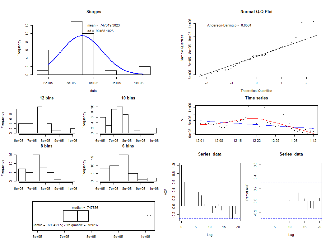
summary.plot <- function(data, xlabels){
    require(nortest)
    require(MASS)
    library(tree)
    library(mgcv)
    # first job is to save the graphics parameters currently used
    def.par <- par(no.readonly = TRUE)
    par("plt" = c(.2,.95,.2,.8))
    layout( matrix(c(1,1,2,2,1,1,2,2,4,5,8,8,6,7,9,10,3,3,9,10), 5, 4, byrow = TRUE))

    #histogram on the top left
    h <- hist(data, breaks = "Sturges", plot = FALSE)
    xfit<-seq(min(data),max(data),length=100)
    yfit<-yfit<-dnorm(xfit,mean=mean(data),sd=sd(data))
    yfit <- yfit*diff(h$mids[1:2])*length(data)
    plot (h, axes = TRUE, main = "Sturges")
    lines(xfit, yfit, col="blue", lwd=2)
    leg1 <- paste("mean = ", round(mean(data), digits = 4))
    leg2 <- paste("sd = ", round(sd(data),digits = 4))
    legend(x = "topright", c(leg1,leg2), bty = "n")

    ## normal qq plot
    qqnorm(data, bty = "n", pch = 20)
    qqline(data)
    p <- ad.test(data)
    leg <- paste("Anderson-Darling p = ", round(as.numeric(p[2]), digits = 4))
    legend(x = "topleft", leg, bty = "n")

    ## boxplot (bottom left)
    boxplot(data, horizontal = TRUE)
    leg1 <- paste("median = ", round(median(data), digits = 4))
    lq <- quantile(data, 0.25)
    leg2 <- paste("q1 =  ", round(lq,digits = 4))
    uq <- quantile(data, 0.75)
    leg3 <- paste("q3 = ", round(uq,digits = 4))
    legend(x = "top", leg1, bty = "n")
    legend(x = "bottom", paste(leg2, leg3, sep = "; "), bty = "n", lty = c(1,2))


    ## the various histograms with different bins
    h2 <- hist(data,  breaks = (0:12 * (max(data) - min (data))/12)+min(data), plot = FALSE)
    plot (h2, axes = TRUE, main = "12 bins")

    h3 <- hist(data,  breaks = (0:10 * (max(data) - min (data))/10)+min(data), plot = FALSE)
    plot (h3, axes = TRUE, main = "10 bins")

    h4 <- hist(data,  breaks = (0:8 * (max(data) - min (data))/8)+min(data), plot = FALSE)
    plot (h4, axes = TRUE, main = "8 bins")

    h5 <- hist(data,  breaks = (0:6 * (max(data) - min (data))/6)+min(data), plot = FALSE)
    plot (h5, axes = TRUE,main = "6 bins")

    ## the time series, ACF and PACF
    #plot (data, main = "Time series", pch = 20)

    x <- xlabels
    y <- data
    #fit1 <- rlm(y~x)
    fit1 <- lqs(y~x, method="lts", quantile=8)
    pred <- predict(fit1, data.frame(x=x))
    lwr <- pred - (IQR(pred)/1.35)*3
    upr <- pred + (IQR(pred)/1.35)*3

    ylim <- c(min(y)*0.9, max(y)*1.1)
    if (min(lwr) < min(y)){
        ylim <- c(min(lwr)*0.9, max(y)*1.1)
    }
    plot(x,y, main="Time series", pch = 20, type="l", ylim=ylim)
    points(x,y, main="Time series", pch = 20)
    lines(x, pred, col="blue")
    lines(x, lwr, col="blue", lty=2)
    lines(x, upr, col="blue", lty=2)
    #lines(x, predict(fit1, data.frame(x=x)), col="blue")
    x <- 1:length(y)
    fit2 <- gam(y~s(x))
    tree.model <- tree(data.frame(y, x))
    pred1 <- predict(tree.model, list(x=x))
    x <- xlabels
    lines(x, pred1, col="red")

    acf(data, lag.max = 20)
    pacf(data, lag.max = 20)

    ## reset the graphics display to default
    par(def.par)
}
[edit]
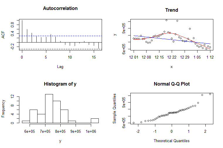
14 4-plot #
four.plot <- function(y, xlabels){
    par(mfrow=c(2,2))

    acf(y, main="Autocorrelation")

    x <- xlabels
    plot(x,y, main="Trend")
    fit1 <- rlm(y~x)
    lines(x, predict(fit1, data.frame(x=x)), col="blue")
    x <- 1:length(y)
    fit2 <- loess(y~x)
    pred <- predict(fit2, data.frame(x=x))
    x <- xlabels
    lines(x, pred, col="red")

    hist(y)
    qqnorm(y)

    par(mfrow=c(1,1))
}
[edit]
15 Robust Z #
robustz <- function(x){
    sigma <- IQR(x)/1.35
    if(sigma == 0) sigma <- sd(x)
    if(sigma == 0) sigma <- 0.0001
    z <- (x - median(x)) / sigma
    return(z)
}
п»ҝ